Example: confidence
Romberg Integration - USM
is approximated using the Composite Trapezoidal Rule with step sizes h k = (b a)2 k, where k is a nonnegative integer. Then, for each k, Richardson extrapolation is used k 1 times to previously computed approximations in order to improve the order of accuracy as much as possible.
Tags:
Information
Domain:
Source:
Link to this page:
Documents from same domain

Orthogonality of Bessel Functions - USM
www.math.usm.eduNormalization Now that we have orthogonal Bessel functions, we seek orthonormal Bessel functions. From Z a 0 ˆ[J (kˆ)]2 dˆ= lim k0!k a[k 0J (ka)J (ka) kJ (ka)J (ka)]
Three-Dimensional Coordinate Systems
www.math.usm.eduJim Lambers MAT 169 Fall Semester 2009-10 Lecture 17 Notes These notes correspond to Section 10.1 in the text. Three-Dimensional Coordinate Systems

Properties of Sturm-Liouville Eigenfunctions and Eigenvalues
www.math.usm.eduReal Eigenvalues Just as a symmetric matrix has real eigenvalues, so does a (self-adjoint) Sturm-Liouville operator. Proposition 2 The eigenvalues of a regular or periodic Sturm-Liouville problem are real.

The Secant Method - USM
www.math.usm.eduJim Lambers MAT 772 Fall Semester 2010-11 Lecture 4 Notes These notes correspond to Sections 1.5 and 1.6 in the text. The Secant Method One drawback of Newton’s method is that it is necessary to evaluate f0(x) at various points, which may not be practical for some choices of f.

Gram-Schmidt Orthogonalization - USM
www.math.usm.edueach polynomial depends on the previous two. Table lists several families of orthogonal polynomials that can be generated from such a recurrence relation; we will see some of these families later in the course. Polynomials Scalar Product Legendre R 1 1 P n(x)P m(x)dx= 2 mn=(2n+ 1) Shifted Legendre R 1 0 P n(x)P m (x)dx= mn=(2n+ 1) Chebyshev ...

The Wronskian - math.usm.edu
www.math.usm.eduWe de ne a second-order linear di erential operator Lby L[y] = y00+ p(t)y0+ q(t)y: Then, a initial value problem with a second-order homogeneous linear ODE can be stated as L[y] = 0; y(t 0) = y 0; y0(t 0) = z 0: We state a result concerning existence and uniqueness of solutions to such ODE, analogous to the Existence-Uniqueness Theorem for rst ...

Linear Interpolating Splines - USM
www.math.usm.eduLinear Interpolating Splines We have seen that high-degree polynomial interpolation can be problematic. However, if the tting function is only required to have a few continuous derivatives, then one can construct a piecewise polynomial to t the data. We now precisely de ne what we mean by a piecewise polynomial.

Gaussian Elimination and Back Substitution
www.math.usm.eduThe process of eliminating variables from the equations, or, equivalently, zeroing entries of the corresponding matrix, in order to reduce the system to upper …
Properties of Sturm-Liouville Eigenfunctions and …
www.math.usm.eduThe following essential result characterizes the behavior of the entire set of eigenvalues of Sturm-Liouville problems. Proposition 6 The set of eigenvalues of a regular Sturm-Liouville problem is countably in nite, and is a monotonically increasing sequence 0 < 1 < 2 < < n< n+1 < with lim n!1 n = 1. The same is true for a periodic Sturm ...
Orthogonality of Bessel Functions - USM
www.math.usm.eduOrthogonality of Bessel Functions Since Bessel functions often appear in solutions of PDE, it is necessary to be able to compute coe cients of series whose terms include Bessel functions. Therefore, we need to understand their orthogonality properties. Consider the Bessel equation ˆ2 d2J (kˆ) dˆ2 + ˆ dJ (kˆ) dˆ + (k2ˆ2 2)J (kˆ) = 0 ...
Related documents

Chapter 07.02 Trapezoidal Rule of Integration
mathforcollege.comTrapezoidal Rule of Integration . After reading this chapter, you should be able to: 1. derive the trapezoidal rule of integration, 2. use the trapezoidal rule of integration to solve problems, 3. derive the multiple-segment trapezoidal rule of integration, 4. use the multiple-segment trapezoidal rule of integration to solve problems, and 5.

simpson's 1/3 rule - MATH FOR COLLEGE
mathforcollege.comThe trapezoidal rule was based on approximating the integrand by a first order polynomial, and then integrating the polynomial interval of integration. Simpson’s 1/3 rule is an . over . 07.03.2 Chapter 07.03 . extension of Trapezoidal rule where the integpproximated by a …

Chapter 5: Numerical Integration and Differentiation
www.ece.mcmaster.caThe trapezoidal rule is equivalent to approximating the area of the trapezoidal Figure 1: Graphical depiction of the trapezoidal rule under the straight line connecting f(a) and f(b). An estimate for the local trun-2

SUGI 27: Using a Trapezoidal Rule for the Area under a ...
support.sas.comThe trapezoidal rule is a numerical integration method to be used to approximate the integral or the area under a curve. The integration of [a, b] from a functional form is divided into n equal pieces, called a trapezoid. Each subinterval is approximated by the integrand of a
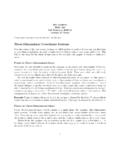
3 Runge-Kutta Methods - IIT
math.iit.edupredictor for the (implicit) trapezoidal rule. We obtain general explicit second-order Runge-Kutta methods by assuming y(t+h) = y(t)+h h b 1k˜ 1 +b 2k˜ 2 i +O(h3) (45) with k˜ 1 = f(t,y) k˜ 2 = f(t+c 2h,y +ha 21k˜ 1). Clearly, this is a generalization of the classical Runge-Kutta method since the choice b 1 = b 2 = 1 2 and c 2 = a 21 = 1 ...
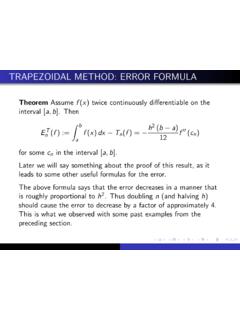
TRAPEZOIDAL METHOD: ERROR FORMULA
homepage.math.uiowa.eduThe corrected trapezoidal rule In general, I(f) T n(f) ˇ h2 12 f0(b) f0(a) I(f) ˇCT n(f) := T n(f) h2 12 f0(b) f0(a) This is the corrected trapezoidal rule. It is easy to obtain from the trapezoidal rule, and in most cases, it converges more rapidly than the trapezoidal rule.

NUMERICAL STABILITY; IMPLICIT METHODS
homepage.math.uiowa.eduTHE TRAPEZOIDAL METHOD The backward Euler method is stable, but still is lacking in accuracy. A similar but more accurate numerical method is the trapezoidal method: y n+1 = y n + h 2 [f (x n;y n) + f (x n+1;y n+1)]; n = 0;1;::: (6) It is derived by applying the simple trapezoidal numerical integration rule to the equation Y(x n+1) = Y(x n) + Z ...

Integration Rules and Techniques - Grove City College
www2.gcc.eduSimpson’s Rule (Quadratic Approximation): Uses a quadratic to approximate the function at the top of the \rectangle" over the corresponding subinterval. Zb a f(x) dxˇS n = x 3 ... T be the errors in the Midpoint and Trapezoidal Approximations, respectively. If jf00(x)j K; a x b then jE Mj K(b a)3 24n2 and jE T j K(b a)3 12n2: Let E
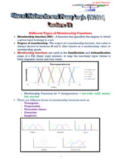
Different Types of Membership Functions
www.philadelphia.edu.joo Trapezoidal membership function: trapmf. Two membership functions are built on the Gaussian distribution curve: a simple Gaussian curve and a two-sided composite of two different Gaussian curves. The two functions are gaussmf and gauss2mf. The generalized bell membership function is specified by three