Second Order Differential Equations - UNCW Faculty and ...

1 3 Second Order Differential EquationsWe now turn to Second Order Differential Equations . Suchequations involve the Second derivative,y (x). Let s assume that we canwrite the equation asy (x) =F(x,y(x),y (x)).We would like to solve this equation using Simulink. This is accomplishedusing two integrators in Order to outputy (x)andy(x).input outputy y (b)input outputyy (a) outputyy input y (c) : Basic schemes for usingIntegrator blocks for solving secondorder Differential shown in (b), sendingy (x)into theIntegratorblock, weget outy (x). This is similar to usingy (x)to gety(x)in (a). Asshown in (c), combining twoIntegratorblocks, we can inputy (x) =F(x,y,y )and get outyandy . Feeding this output intoF(x,y,y ),we then obtain a model for solving the Second Order Differential general schematic for solving an initial value problem of the formy =F(x,y,y ),y(0) =y0,y (0) =v0, is shown in outputyy y F(x,y,y )y (0)y(0) : This is a general schematicfor solving an initial value problem ofthe formy =F(x,y,y ),y(0) =y0,y (0) = this chapter we will demonstrate the modeling of Second Order con-stant coefficient Differential Equations and show some simple solving Differential Equations using Coefficient EquationsWe can solve Second Order constant coefficient differentialequationsusing a pair of integrators.

2 An example is displayed in Here we solve the constant coefficient Differential equationay +by +cy=0by first rewriting the equation asy =F(y,y ) = bay the initial value problemy +5y +6y=0,y(0) =0,y (0) =1,in simulation in the equationy +5y +6y=0with appropriate initial conditions. There are two integrators. Oneintegrates the first input,y , and the other integrates the output ofthe first integrator,y , giving an output ofy. EachIntegratorblockneeds an initial condition. The first takesy (0) =1 and the secondneedsy(0) = 'yy''b/a y'c/a ySecond Order Constant Coefficient ODE1sIntegrator1sIntegrator15b/a6 : Model for the Second orderconstant coefficient ODEy +5y +6y= outputs,yandy are multiplied by the appropriate constantsusing aGainblock. They are then combined to form the input,F(y,y ) = 5y 6y, to the system of integrators.

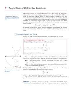
3 Running thesimulation for5units of time, the Scope gives the solution shown Solutionsecond Order Differential Equations (x) vs : Solution plot for the initialvalue problemy +5y +6y=0,y(0) =0,y (0) =1 using the solution of this problem is found by first seeking thetwo linearly independent solutions. Assuming solutions of the formy(x) =erx, the characteristic equation isr2+5r+6= roots of the equation arer= 2, 3. Therefore, the two linearlyindependent solutions arey1(x) =e 2xandy2(x) =e 3x. Thegeneral solution isy(x) =c1e 2x+c2e initial conditions hold if0=c1+c2,1= 2c1 ,c1=1 andc2= 1. The solution to the initial value problem isy(x) =e 2x e plot of this solution is shown in It is seen to agreewith the solution shown in : Plot of the exact solutionof the initial value problemy +5y +6y=0,y(0) =0,y (0) = OscillationIn the following we will suppress SI units the mass is in kilograms(kg), displacementxis in meters (m),and force is in Newtons (N).

4 Then,khas units of N/m. One could alsouse CGS units of g, cm, dynes, anddynes/cm, respectively. Time unitswill generally be in seconds, leavingfrequencies in s 1, or Hertz (Hz).A typical application of Second Order , constant coefficient Differential equa-tions is the simple harmonic oscillator as shown in Considera mass,m, attached to a spring with spring constant,k. According to46 solving Differential Equations using simulinkHooke s law, a stretched spring will react with a forceF= kx, wherexis the displacement of the spring from its unstretched equilibrium. Themass experiences a net for and will accelerate according to Newton s Sec-ond Law of Motion,F=ma. Setting these forces equal and noting thata= x, we havem x+kx= : A simple harmonic oscillatorconsists of a mass,m, attached to aspring with spring constant, we assume thatx=x(t)and let the derivatives be time deriva-tives.

5 The characteristic equation is given bymr2+k=0, orr= i km i , the general solution is given asx(t) =Acos 0t+Bsin will model the equation for simple harmonic motion and it varia-tions in the next examples. Namely, we will look at Simulink examples ofsimple harmonic motion, damped harmonic motion, and forced Harmonic MotionA Simulink model for simple harmonic motion is shown in We write the Differential equation in the form x= 1m(kx).For this example we setk=5 andm=2. We also specify the initialconditionsx(0) =1 and x(0) =0 in the two Harmonic Oscillatorx'xx''1sIntegrator1sIntegrator 15kScope1-1/2-1 : A model for simple har-monic motion,m x+kx= output on the scope is shown in [0, 10].Solving the initial value problem we find thatx(t) =cos 0t, where 0= km= , the period isT=2 0 might have estimated the period Order Differential Equations 47 Time offset:0 : Output for the solution ofthe simple harmonic oscillator Simple Harmonic MotionA simple modification of the harmonic oscillator is obtained byadding a damping term proportional to the velocity, x.

6 This results inthe Differential equationm x+b x+kx=0,whereb>0 is the damping can verify the damping behavior in the solution by studyingthe characteristic equation,mr2+br+k=0,wherex(t) =ertis a guess for form of the the linearly independentsolutions. The solutions of the characteristic equation are foundusing the quadratic formula,r= b b2 4km<0, then the roots of the characteristic equation arecomplex conjugate roots and the solution takes the formx(t) =e bt/2m[Acos 0t+Bsin 0t],where 0= 4km this case one has oscillatroy solutions with an exponentially decay-ing Simulink model for the damped harmonic oscillator can becreated using the Differential equation in the form x= 1m(b x+kx).This leads to a modification of the model in We simplyadd a termb x. The model is shown in consider a specific example usingk=5,m=2, andb= initial conditionsx(0) =1 and x(0) =0 are used in the two48 solving Differential Equations using simulinkDamped Oscillatorx'xx'' : A model for damped simpleharmonic motion,m x+b x+kx= offset:0 : Output for the solution ofthe damped harmonic oscillator Running the model fort [0, 20], the solution seen in theScopeblock is shown in We note that 0= Hz,or the period of oscillation isT= This is consistent with theSimulink the initial conditions,x(0) =1 and x(0) =0, to thegeneral solution, we find thatA=1 and0= b2mA+ 0B, orB=b2m 0.

7 ( )Therefore, the particular solution of the initial value problem can bewritten asx(t) =e bt/2m[cos 0t+b2m 0sin 0t].For the parameter values in the problem a plot of this oslution isshown in agrees with this plot in obtained using MATLAB sezplotfunction and it symbolic capability. The code is given below for tsecond Order Differential Equations Harmonic : The analytic solutionfor the damped harmonic ; m=2; k=5;omega=sqrt(4*k*m-b^2)/2/m;alpha=b/2/ m;A=1;B=b/(2*m*omega);x=exp(-alpha*t)*(A *cos(omega*t)+B*sin(omega*t));ezplot(x,[ 0,20]);title( Damped Harmonic Motion )Another modification of the problem is to introduce forcing. In general,the corresponding nonhomogeneous equation ism x+b x+kx=f(t). Oneneed only addf(t)to the sum that is sent into the also requires theClockblock and some function blocks.

8 We show thisin the next Simple Harmonic MotionWe consider a simple sinusoidal forcing and no damping given bym x+kx=F0sin Simulink model in modified to produce the modelin adding aSine Wave Functionand aClock. We leftthe dampingGainblock but set the multiplier to zero. We also notethat theSumblock shape was changed to rectangular to accommo-date more inputs and to direct a consistent flow of the the constantsm=2,k=10, we setF0=1 and =2 in theSine Wave Function. This results in the output shown in that the solution is a modulated oscillation. This is understoodfrom looking at the analytic form of the that we can obtain the analytic solution to this problem us-ing the Method of Undetermined Coefficients. The general solution50 solving Differential Equations using simulinkForced Oscillatorx'xx''1sIntegrator1sIntegrator 10b10kScope11/21/mtSine : A model for forced simpleharmonic motion,m x+kx=sin offset:0 : Output for the solution ofthe forced simple harmonic a solution of the homogeneous problem plus a particular solution,or guess, to the nonhomogeneous problem.

9 Thus, we havex(t) =Acos 0t+Bsin 0t+xp(t).We make an educated guess for a functionxp(t)satisfyingm xp+kxp=F0sin that two derivatives of a sine function returns a constanttimes the sine function, we assume thatxp(t) =asin t, providingthat this is not a solution of the homogeneous problem. Namely, 6= this guess into the Differential equation, we have m 2asin t+kasin t=F0sin this is true for allt, m 2a+ka=F0. Noting thatk=m 20, wecan solve fora,a=F0m( 20 2).Then, the general solution is given byx(t) =Acos 0t+Bsin 0t+F0m( 20 2)sin t, 6= Order Differential Equations 51 The initial conditions,x(0) =1 and x(0) =0, were again usedin the two integrators. The first condition givesA=1. The secondcondition can be written as0= 0B+F0 m( 20 2).Solving forB, we obtainB= F0 m 0( 20 2).

10 Harmonic : The analytic solution forthe forced harmonic oscillator the constants1in this problem, the exact solution to the1 Recall thatm=2,k=10,F0=1, =2. Therefore, 0= k/m= value problem is found asx(t) =12sin 2t+cos 5t 1 5sin plot of this solution is in It agrees with that given bythe Simulink model in a modulation form of the solution from showing how to derive a modu-lated form,x(t) =C( (t))sin( (t) + ).The solution,x(t) =12sin 2t+cos 5t 1 5sin 5t,( )in like what one would get when adding sinusoidalfunctions with frequencies that are close. It is the principle used bypiano tuners when using a tuning fork to tune a piano key. If thepiano key note is slightly different from that of a tuning fork, thenwhen both are sounded at the same time, one hears a beat is heard as the low frequency of the envelope similar to that In the last example we had two frequencies, =2 and 0= 5 , which were close solving Differential Equations using simulinkWe will combine the the trigonometric functions in Equation ( )and show the root of this modulation.