Search results with tag "Second order differential equations"
Application of Second Order Differential Equations in ...
www.engr.sjsu.eduReview solution method of second order, non-homogeneous ordinary differential equations - Applications in forced vibration analysis ... Review Solution Method of Second Order, Homogeneous Ordinary Differential Equations. Typical form ( ) 0 ( ) ( ) 2 2 + +bu x = dx du x a dx d u x (4.1) where a and b in Equation (4.1) are constants The solution ...
Chapter Second Order Differential Equations
people.uncw.eduChapter 2 Second Order Differential Equations “Either mathematics is too big for the human mind or the human mind is more than a machine.” - Kurt Gödel (1906-1978)2.1 Introduction In the last section we saw how second order differential equations

MATHEMATICS
cisce.orgDifferential equations, order and degree. -Solution of differential equations. -Variable sep arable. NOTE-Homogeneous equations. - = Linear form. Py Q dx dy + where P and Q are functions of x only. Similarly, for dx/d. y. NOTE : The second order differential equations are excluded. 4. Probability. Conditional probability, multiplication theorem
MODELING FIRST AND SECOND ORDER SYSTEMS IN …
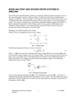
www.science.smith.eduMODELING FIRST AND SECOND ORDER SYSTEMS IN SIMULINK First and second order differential equations are commonly studied in Dynamic Systems courses, as they occur frequently in practice. Because of this, we will discuss the basics of modeling these equations in Simulink. The first example is a low-pass RC Circuit that is often used as a filter.
Second Order Differential Equations
epsassets.manchester.ac.uk1. Constant coefficient second order linear ODEs We now proceed to study those second order linear equations which have constant coefficients. The general form of such an equation is: a d2y dx2 +b dy dx +cy = f(x) (3) where a,b,c are constants. The homogeneous form of (3) is the case when f(x) ≡ 0: a d2y dx2 +b dy dx +cy = 0 (4)
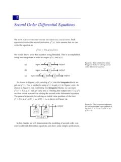
Second Order Differential Equations
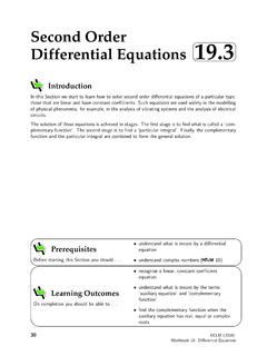
people.uncw.edusecond order differential equations 45 x 0 0.5 1 1.5 2 2.5 3 3.5 4 4.5 5 y 0 0.05 0.1 0.15 y(x) vs x Figure 3.4: Solution plot for the initial value problem y00+ 5y0+ 6y = 0, y(0) = 0, y0(0) = 1 using Simulink. Recall the solution of this problem is found by first seeking the