MODELING FIRST AND SECOND ORDER SYSTEMS IN …

1 MODELING FIRST AND SECOND ORDER SYSTEMS IN SIMULINK FIRST and SECOND ORDER differential equations are commonly studied in Dynamic SYSTEMS courses, as they occur frequently in practice. Because of this, we will discuss the basics of MODELING these equations in Simulink. The FIRST example is a low-pass RC Circuit that is often used as a filter. This is modeled using a FIRST - ORDER differential equation. The SECOND example is a mass-spring-dashpot system . This system is modeled with a SECOND - ORDER differential equation (equation of motion).

2 To better understand the dynamics of both of these SYSTEMS were are going to build models using Simulink as discussed below. You should build both models FIRST , then run them so you can compare how each system responds to the same input. MODELING a FIRST ORDER Equation (RC Circuit) The RC Circuit is schematically shown in Fig. 1 below. RCVin Vout Fig. 1. The RC Circuit. The differential equation for this is as show in (1) below. [x)t(fRC1x =&] (1) Where (xdot) is the time rate of change of the output voltage, R and C are constants, f(t) is the forcing function (Input voltage), and x is the output voltage.

3 We are now going to take this piece by piece. FIRST , we examine what is in the brackets and we notice that we are subtracting the term x from the term f(t). If we imagine that each of these terms outputs a signal, we can model this relationship as shown in Fig. 2 below. x& Fig. 2. Summing the input signals. Now we notice that the bracketed term [f(t) x] is multiplied by a constant 1/RC. We do this in Simulink by passing the signal through a Gain block as in Fig. 3 below. Because all the terms on the right-side of xdot are accounted for, we know that the output signal must be equal to the left side of the equation, which is xdot.

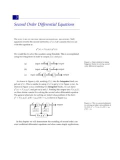
4 MODELING FIRST and SECOND ORDER 1 rev. 090604 SYSTEMS Fig. 3. Applying a gain to the output. However, we are interested in x, not xdot. How can we take the xdot output signal and get an x output? The answer is to use an integrator block as in Fig. 4 below. Fig. 4. Integrating the output signal. Now, we have the desired x output, but we notice that x is also an input of the system . In our model above, the input x branch is a dead branch. In other words, there is no real signal going in there. How can we make x both an output and input of the system ?

5 The answer is to use a feedback loop by tapping the output x signal and feeding it back into the system at the input point. After some manipulation of the lines, your model should look like Fig. 5 below. Fig. 5. The finished Simulink model. After adding a Scope block, you are ready to set the block parameters, and run the simulation. But FIRST , take the time to build the SECOND - ORDER model as described in the following section. MODELING a SECOND ORDER Equation (Single Degree of Freedom system -SDOF) The mass-spring-dashpot is a basic model used widely in mechanical engineering design to model real-world mechanical SYSTEMS .

6 It is represented schematically as shown in Fig. 6 below. mk c Fig. 6. The SDOF Mass-Spring-Dashpot. The response of this system is governed by the equation of motion which is a SECOND - ORDER differential equation, and is shown in (2) below MODELING FIRST and SECOND ORDER 2 rev. 090604 SYSTEMS []kxxc)t(fm1x =&&& (2) Where (xddot) is the acceleration of the mass m, (xdot) is the velocity, x is the displacement, f(t) is the forcing function (input force), c is the damping coefficient, and k is the spring constant.

7 X&&x& To model this system we start by looking at the terms in the bracket. There are three input signal lines: f(t), xdot, and x. We also notice that both xdot and x are multiplied by constants. As in the case of the FIRST - ORDER model; this can be done in Simulink by using a Gain block. The signals are then summed together as in Fig. 7 below. Fig. 7. Summing the input signals. Now, we notice that the bracketed term [f(t)- cxdot- kx] is multiplied by the constant 1/m. We do this in by passing the signal through a Gain block as in Fig.

8 8 below. Fig. 8. Applying a gain to the output. Again, we are interested in the displacement x, not xddot. To get the x output signal we integrate the xddot output signal twice, as in Fig. 9 below. Fig. 9. Integrating the output signal twice. MODELING FIRST and SECOND ORDER 3 rev. 090604 SYSTEMS We can see from the model that xdot and x are both outputs and inputs of the model. Therefore, we need to use a feedback loop for each of these signals as discussed in the FIRST ORDER model example. The resulting model should look like Fig.

9 10 below. Fig. 10. The finished Simulink model for a SDOF system . Before running the model be sure to include a Scope block for viewing the results. Now that the model is complete, we are ready to run the simulation and look at the results. Running Simulation and Analyzing data Having completed the Simulink Models for both the FIRST and SECOND ORDER SYSTEMS , it is now time to run a simple simulation and look at the results. We will start FIRST with the FIRST - ORDER system , and then show the simulation and results for the SECOND - ORDER system .

10 FIRST ORDER differential Equation (RC Circuit) Double-click on the Integrator block and set the initial conditions to zero as shown in Fig. 11 Leave the remaining fields as they are. Fig. 11. Integrator block parameters Now, double click on the Gain block and set the gain to the values shown in Fig. 12 below. MODELING FIRST and SECOND ORDER 4 rev. 090604 SYSTEMS Fig. 12. Gain block parameters Open the Step block to familiarize yourself with the parameters. Now, run the simulation and open the Scope block.