Transcription of Second-Order LTI Systems
1 Engineering Sciences 22 Systems 2nd order Systems Handout Page 1 Second-Order LTI Systems First order LTI Systems with constant, step, or zero inputs have simple exponential responses that we can characterize just with a time constant. second order Systems are considerably more complicated, but are just as important, and are more interesting. We won't find a super-simple shortcut for finding solutions the Laplace transform is usually the way to go. But we will gain a lot of insight. second order system Consider a typical Second-Order LTI system , which we might write as )()()()(21tbtyktykty=++&&&, where b(t) is some input function.
2 (Not all second order LTI Systems have exactly this same form this is just a common example.) Solution by Laplace transform substituting yields )()()0()()0()0()(2112sBsYkykssYkysysYs=+ + & which we solve for Y(s) )()0()0()0())((1212sBykysykskssY+++=++& )()()0()0()0()(2121kskssBykysysY+++++=& The solution to this depends on what the input b(t) is, as well as the initial conditions. But in any case we can re-write the denominator in factored form: ))(()()0()0()0()(1bsassBykysysY+++++=& where -a and -b are the roots of the denominator polynomial, also called the "characteristic equation".
3 The roots -a and -b are also called the poles of Y(s); the values of s where Y(s) goes to infinity. Engineering Sciences 22 Systems 2nd order Systems Handout Page 2 Some of the common possibilities for Y(s) are given in table entries 10-14. (If the input is constant, zero, or a step, Y(s) will in fact be one of these, or a combination of them, depending on initial conditions.) We observe that all of the corresponding solutions y(t) can be described by y(t)=C+Ae at+Be bt where A, B, and C are constants.
4 Thus, the solutions are like the first- order solution, but with two exponential terms, instead of just one. We will now study the behavior as a function of the values of the roots (poles), -a and -b. We can divide the possibilities into three cases: two distinct real poles, two equal real poles, or a complex conjugate pair of poles. Case 1: Distinct Real Roots The response usually looks like a first- order exponential response. In fact, if A and B have the same sign and the poles are close to each other, it can be nearly indistinguishable from an exponential response.
5 However, careful examination can often show differences that are not immediately visible. In Fig. 1 we see an example of a second order response, y(t)= t/2+ 2t. At first it looks like a simple exponential decay. It looks like the time constant is 1, because the response is down to 37% there. But a simple first- order exponential would be down to 5% at three time constants, and at t = 3, it is only down to about 11%. So the general shape is similar, but it is a different shape. (t)2nd- order response1st- order response Fig.
6 1. First vs. Second-Order responses. However, it can also look quite different. The responses with different parameter values, y(t)=1+e t 2e 4t and y(t)= t/4+ 4t are shown in Fig. 2. The first gives a response with "overshoot." The second gives a response with a distinct knee; the transition from the rapid decay of the last term to the y(t) Engineering Sciences 22 Systems 2nd order Systems Handout Page 3 slow decay of the first. In homework two you solved a Second-Order system with ode45 and saw a response very similar to this curve with a knee.
7 (t) Case 2: Two Real Roots, exactly equal This case is of little practical importance, because in practice you can't ever get the roots to match exactly. Thus, it won't be discussed further here. If you ever need to analyze this case you can use table entries 34 and 35. Case 3: Two Complex Conjugate Roots y(t)=C+Ae at+Be bt with b = a*. Define: Re(a)=Re(b)= Re(p1)= Re(p2) (1) and: d Im(a)= Im(b) (2) such that a,b{}= j d Now y(t)=C+Ae t j dt+Be t+j dt y(t)=C+e tAe j dt+Bej dt() We can apply Euler's formula (ejx=cosx+jsinx) to rewrite this as y(t)=C+e t(A+B)cos dt+(B A)jsin dt() (3) The solution (3)
8 Is a little disconcerting, because it looks like the solution could be complex. If it was a solution for a position of an object, a complex value wouldn't be physically meaningful. For example, what if B = -A, so the cosine term was zero, and we had only the imaginary sine term!? Actually, B and A are complex, and are related to a and b, so it isn't so simple to see what happens, but it turns out that with a and b complex conjugates, (B-A) is always pure imaginary or zero, so the sine term always becomes real after all.
9 (Try an example from the table to see this.) Engineering Sciences 22 Systems 2nd order Systems Handout Page 4 Thus, we can write the solution as y(t)=C+e tDcos dt+Esin dt() or y(t)=C+A0e tcos dt+ () (4) In these expressions, C, D, E, A0 and are real constants that we haven't explicitly found yet, and and d are real constants that can be determined from the poles (see eqns (1) and (2)).
10 Further Study of Case 3: Two Complex Conjugate Roots From (4), we see that the response comprises a decaying sinusoidal oscillation. The frequency of this decaying or damped oscillation is d radians per second , or d/( 2 ) Hz. The decay rate is . These two numbers correspond to the horizontal and vertical positions of the poles on the complex plane. Since these are the values of s that make Y(s) go to infinity, we usually refer to this complex plane as the s-plane. Let's look at how the values on the s-plane and the responses correspond.