Transcription of Chapter 2
1 Chapter The Diffusion EquationFormulationAs we saw in the previous Chapter , the flux of a substance consists of anadvective component, due to the mean motion of the carrying fluid, and of aso-called diffusive component, caused by the unresolved random motions of thefluid (molecular agitation and/or turbulence). In this Chapter , we explore someconsequences of the existence of a diffusive flux by concentrating on cases inwhich there is no mean flow in the system and thus investigating the effectscaused by concentration variations across the mass balance on an infinitesimal stretch of a one-dimensional system(Figure 2-1 a river, for example) yields:Vdcdt= Import Export =q(x, t)A q(x+ x, t)A,where the volume of the element isV=A x, and the Import and Export aresimply the flux times the cross-sectional area.
2 The preceding equation can berewritten as:Figure control volume in one 2. DIFFUSION dcdt= q(x+ x, t) q(x, t) x,and in the limit of an infinitesimally small stretch x, c t= q x.( )(A switch from total to partial derivatives was necessary since at this stagethere is more than one independent variables.)It is important to note that the above equation, being a simple mass bal-ance, is valid regardless of whether the fluxqis purely diffusive or containsan advective component. In the absence of a transporting flow(u= 0), thesubstance flux given by ( ), withjgiven by ( ), reduces to:q= D c x,( )which is the diffusive flux caused by the unresolved fluctuating motions suchas those caused by turbulence. We suppose that the diffusion coefficientDisknown.
3 After elimination ofq, Equation ( ) contains the single unknownc: c t= x(D c x).( )This equation is called the one-dimensional diffusion equation or Fick s secondlaw. It can be solved for the spatially and temporally varying concentrationc(x, t) with sufficient initial and boundary general, the diffusion coefficientDmay vary with the local condition ofturbulence, but an interesting case is, of course, that of a constantD: c t=D 2c x2.( )Initial and boundary conditionsThe above diffusion equation is hardly solved in any general way. Eachsolution depends critically on boundary and initial conditions specific to theproblem at and foremost, we need to know how many initial and boundary con-ditions are necessary so that the problem is neither underspecified or overspec-ified.
4 For this, we determine the order of the problem s governing time derivative ( c/ t) is of first order and thus calls for a single initialcondition (at allxvalues); typically, the initial concentration distribution isgivenc=c0(x) att= 0.( ) DIFFUSION EQUATION27 The spatial derivative ( 2c/ x2) is of second order and thus calls for two bound-ary conditions; typically, any problem will include one boundary condition ateach end of the domain (sayx=x1andx=x2). While it would be easierfrom a mathematical perspective to have the end concentrations imposed, forexample,c=c1(t) atx=x1( )c=c2(t) atx=x2,( )it is much more typical to encounter flux boundary conditions D c x=q1atx=x1( ) D c x=q2atx=x2.( )An impermeable boundary implies no flux and thus no concentration gradientat that boundary.
5 Of course, mixed conditions ( , concentration given atone end of the domain and flux specified at the other) are a first example showing how a diffusion problem may be solvedanalyti-cally, we shall now derive the solution to an ideal but most important solutionThe diffusion equation is a linear one, and a solution can, therefore, beobtained by adding several other solutions. An elementary solution ( buildingblock ) that is particularly useful is the solution to an instantaneous, localizedrelease in an infinite domain initially free of the , the problem is stated as follows: Infinite domain: < x <+ , D= constant, No initial concentration, except for the localized release:c0(x) =M (x) att= 0. Since the substance will take an infinite time to reach the infinitely far endsof the domain, we impose:limx + c= limx c= 0at finite times (t < ).
6 In the above,Mis the total mass of the substance released per unit cross-sectional area, and (x) is the Dirac function [ (x) = 0 forx6= 0, (x) = + atx= 0, and area under the infinitely tall and infinitely narrow peak is unity].Physically, we anticipate a behavior as displayed in Figure2-2. The pol-lutant patch gradually spreads on both sides of the release location, with acommensurate decrease in the maximum center value. Curves at later times28 Chapter 2. DIFFUSIONF igure in time of an initially localized pollutant the pollution patch spreads, the maximum concentration decreases, pre-serving the area under the similar to those at earlier times, only being flatter and wider. Antici-pating such similarity in the solution, we write:c(x, t) =t F( ) with =x24Dt,( )wheret (with the dimensionless exponent expected to be positive) is a sizefactor to represent the temporal decay of the maximum concentration value(atx= 0), and where the functionF( ) is the shape factor giving the similarcurve profile.
7 This function has a stretched coordinate sothat the same valueF( ) is obtained for increasing values ofxas time goes on (constantx2/t). Thisis to take into account the spreading of the pollutant exponent 2 ofxis an educated guess, to render the functional dependency compatible withthe equation at hand. [The choice is rooted in the fact thattappears in theequation as a first-order derivative, whilexenters the equation as a second-order derivative.] The factorDin the denominator of is there to make theratio dimensionless; therefore has no units, and its functionF( ) takes on auniversal character. Finally, the factor 4 is introduced for pure DIFFUSION ( ), we calculate the derivatives ofcneeded to solve Equation ( ): c t= t 1F( ) +t dFd t= t 1F( ) t 1dFd c x=t dFd x=xt 12 DdFd 2c x2=t 12 DdFd +xt 12Dd2Fd 2 x=t 12 DdFd +t 1D d2Fd , substitution of c/ tand 2c/ x2in the diffusion equation yields: t 1F( ) t 1dFd =12t 1dFd + t 1d2Fd time factors cancel out (thanks to the careful definitionof ), and thepartial-differential equation is reduced to an ordinary differential equation, withvariable : dd (dFd +F)+12(dFd + 2 F)= 0.
8 ( )Since the exponent is still free, we will now choose it so that the two groupsin the parentheses are identical, = 1/2. A solution is one that obeysdFd +F( ) = 0,which is:F( ) =Ae ,whereAis an arbitrary constant of all the pieces together, we arrive at the following solution:c(x, t) =At 1/2exp( x24Dt).We note that this solution already meets the boundary conditions (vanishingconcentrations far away on both sides). The remaining, initial condition de-termines the constant of integration. Conservation of the total amount of thesubstance requires that + c(x, t)dx= + c0(x)dx=Mat all times. Calculations yieldA=M/ 4 D, and the final solution is there-fore:30 Chapter 2. DIFFUSIONc(x, t) =M 4 Dtexp( x24Dt).( )Let us now verify not only that the amount of substance is right but also thatthe initial profile is the peak distribution withc= 0 forx6= 0 andc= forx= 0.
9 Forx6= 0 and fixed, the ratiox2/4 Dtincreases toward infinity astgoesto zero, and the exponential goes to zero. Since the exponential function goesto zero faster thant 1/2goes to infinity, the limit isc 0 fort 0. Atx= 0,however,x2/4Dt= 0, and the exponential is unity;c(0, t) behaves ast 1/2andgoes to infinity astgoes to zero. Thus, expression ( ) satisfies the originalequation, ( ), meets the boundary and initial conditions, and is therefore thecorrect solution to the stated problem. A graphical representation is shown inFigure shall now demystify this solution by deriving it from a totally differentangle, the random-walk Random-Walk ModelRandom-walk processIn one of his celebrated papers of 1905, Albert Einstein showed that arandom-walk process representing Brownian motion in a gas was mathemati-cally equivalent to Fickian diffusion1.
10 Here, we present a very simplified formof this analogy between diffusion and random a one-dimensional domain (1D axis), divide it in a series of boxes ofidentical lengths ( bins ), and place one particle in one ofthe bins (Figure 2-3).Imagine now that this particle is endowed with a mechanism that makes itjump randomly every time interval, t, according to the following rules: there is a 25% chance that the particle will hop one bin to the left, there is a 25% chance that it will hop one bin to the right, and there is a 50% chance that it will remain in the same bin.[This is the 1D version of the more general 2D random walk, commonly referredto as the drunkard s path: Late into the night, an inebriatedfellow leaves a barand has no recollection of where he is and where he is going; every second or so,he makes a step forward, backward (he turns completely around), leftward orrightward, making a random path that may look like that displayed on Figure2-4.]