Transcription of SECTION 19
1 CONTROL SYSTEMSC ontrol is used to modify the behavior of a system so it behaves in a specific desirable way over time. Forexample, we may want the speed of a car on the highway to remain as close as possible to 60 miles per hourin spite of possible hills or adverse wind; or we may want an aircraft to follow a desired altitude, heading,and velocity profile independent of wind gusts; or we may want the temperature and pressure in a reactorvessel in a chemical process plant to be maintained at desired levels. All these are being accomplished todayby control methods and the above are examples of what automatic control systems are designed to do,without human intervention. Control is used whenever quantities such as speed, altitude, temperature, orvoltage must be made to behave in some desirable way over SECTION provides an introduction to control system design methods.
2 , This SECTION :CHAPTER CONTROL SYSTEM Role of Control Differential Variable OF DYNAMICAL Response, Modes and of First and Second Order Response Performance Specifications for a Second Order Underdamped of Additional Poles and CONTROL DESIGN Specifications and Design Strategy of Control DESIGN Feedback and Observer 06:08:2004 6:43 PM Page Electronics Engineers' Handbook, 5th Edition McGraw-Hill, SECTION 19, pp. , ANALYSIS AND DESIGN : OPEN AND CLOSED LOOP the CD-ROM: A Brief Review of the Laplace Transform, by the authors of this SECTION , examines its use fulness incontrol 06:08:2004 6:43 PM Page SYSTEM DESIGNP anus Antsaklis, Zhiqiany GaoINTRODUCTIONTo gain some insight into how an automatic control system operates we shall briefly examine the speed con-trol mechanism in a is perhaps instructive to consider first how a typical driver may control the car speed over uneven ter-rain.
3 The driver, by carefully observing the speedometer, and appropriately increasing or decreasing the fuelflow to the engine, using the gas pedal, can maintain the speed quite accurately. Higher accuracy can perhapsbe achieved by looking ahead to anticipate road inclines. An automatic speed control system, also calledcruise control, works by using the difference, or error, between the actual and desired speeds and knowledgeof the car s response to fuel increases and decreases to calculate via some algorithm an appropriate gas pedalposition, so to drive the speed error to zero. This decision process is called a control lawand it is implementedin the controller. The system configuration is shown in Fig. The car dynamics of interest are capturedin the plant. Information about the actual speed is fed back to the controller by sensors, and the control deci-sions are implemented via a device, the actuator, that changes the position of the gas pedal.
4 The knowledgeof the car s response to fuel increases and decreases is most often captured in a mathematical in an automobile today there are many more automatic control systems such as the antilock brakesystem (ABS), emission control, and tracking control. The use of feedback control preceded control theory ,outlined in the following sections, by over 2000 years. The first feedback device on record is the famous WaterClock of Ktesibios in Alexandria, Egypt, from the third century ControlThe proportional-integral-derivative (PID) controller, defined by(1)is a particularly useful control approach that was invented over 80 years ago. Here KP, KI, and KDare controllerparameters to be selected, often by trial and error or by the use of a lookup table in industry practice. The goal,as in the cruise control example, is to drive the error to zero in a desirable manner.
5 All three terms Eq. (1) haveexplicit physical meanings in that eis the current error, eis the accumulated error, and represents the , together with the basic understanding of the causal relationship between the control signal (u) and theoutput (y), forms the basis for engineers to tune, or adjust, the controller parameters to meet the design spec-ifications. This intuitive design, as it turns out, is sufficient for many control this day, PID control is still the predominant method in industry and is found in over 95 percent of indus-trial applications. Its success can be attributed to the simplicity, efficiency, and effectiveness of this method. eu KeKeKePID=+ + 06:08:2004 6:43 PM Page Role of Control TheoryTo design a controller that makes a system behave in a desirable manner, we need a way to predict the behav-ior of the quantities of interest over time, specifically how they change in response to different models are most oftenly used to predict future behavior, and control system design methodolo-gies are based on such models.
6 Understanding control theory requires engineers to be well versed in basicmathematical concepts and skills, such as solving differential equations and using Laplace transform. The roleof control theory is to help us gain insight on how and why feedback control systems work and how to sys-tematicallydeal with various design and analysis issues. Specifically, the following issues are of both practi-cal importance and theoretical and stability margins of closed-loop fast and smooth the error between the output and the set point is driven to well the control system handles unexpected external disturbances, sensor noises, and internal the following, modeling and analysis are first introduced, followed by an overview of the classical designmethods for single-input single-output plants, design evaluation methods, and implementation design methods are then briefly presented.
7 Finally, For the sake of simplicity and brevity, the dis-cussion is restricted to linear, time invariant systems. Results maybe found in the literature for the cases of lin-ear, time-varying systems, and also for nonlinear systems, systems with delays, systems described by partialdifferential equations, and so on; these results, however, tend to be more restricted and case DESCRIPTIONSM athematical models of physical processes are the foundations of control theory . The existing analysis andsynthesis tools are all based on certain types of mathematical descriptions of the systems to be controlled, alsocalled plants. Most require that the plants are linear, causal, and time invariant. Three different mathematicalmodels for such plants, namely, linear ordinary differential equation, state variable or state space description,and transfer function are introduced Differential EquationsIn control system design the most common mathematical models of the behavior of interest are, in the timedomain, linear ordinary differential equations with constant coefficients, and in the frequency or transformdomain, transfer functions obtained from time domain descriptions via Laplace models of dynamic processes are often derived using physical laws such as Newton s andKirchhoff s.
8 As an example consider first a simple mechanical system, a spring/mass/damper. It consists of aweight mon a spring with spring constant k, its motion damped by friction with coefficient f(Fig. ). SYSTEMSFIGURE control configuration with cruise control as an 06:08:2004 6:43 PM Page SYSTEM DESIGN y(t) is the displacement from the resting position and u(t) is the force applied, it can be shown usingNewton s law that the motion is described by the following linear, ordinary differential equation with constantcoefficients:where with initial conditionsNote that in the next subsection the trajectory y(t) is determined, in terms of the system parameters, the initialconditions, and the applied input force u(t), using a methodology based on Laplace transform. The Laplacetransform is briefly reviewed in Appendix a second example consider an electric RLC circuit with i(t) the input current of a current source, andv(t) the output voltage across a load resistance R.
9 (Fig. )Using Kirchhoff s laws one may derive:which describes the dependence of the output voltage v(t) to the input current i(t). Given i(t) for t 0, the ini-tial values v(0) and (0) must also be given to uniquely define v(t) for t is important to note the similarity between the two differential equations that describe the behavior of amechanical and an electrical system, respectively. Although the interpretation of the variables is completely differ-ent, their relations described by the same linear, second-order differential equation with constant coefficients. Thisfact is well understood and leads to the study of mechanical, thermal, fluid systems via convenient electric Variable DescriptionsInstead of working with many different types of higher-order differential equations that describe the behavior ofthe system, it is possible to work with an equivalent set of standardized first-order vector differential equationsthat can be derived in a systematic way.
10 To illustrate, consider the spring/mass/damper example. Let x1(t) =y(t),x2(t) =(t) be new variables, called state variables. Then the system is equivalently described by the equationsxt xtxtfmxtkmxtmu122211()()()()()== +and(()t y v () ()()()vtRLvtLCvtRLCit++ =1ytyydy tdtdydtytt()( )()( )()===== ==000000andyy1 ()()y tdy t dt= / () ()()()ytfmytkmytmut++=1 FIGURE , mass, and damper 06:08:2004 6:43 PM Page initial conditions x1(0) =y0and x2(0) =y1. Since y(t) is of interest, the output equation y(t) =x1(t) is alsoadded. These can be written aswhich are of the general formHere x(t) is a 2 1 vector (a column vector) with elements the two state variables x1(t) and x2(t). It is calledthe state vector. The variable u(t) is the inputand y(t) is the outputof the system. The first equation is a vec-tor differential equation called the state equation.)