Transcription of SIGNAL PROCESSING FOR EFFECTIVE VIBRATION …
1 SIGNAL PROCESSING FOR EFFECTIVE VIBRATION analysis . Dennis H. Shreve IRD Mechanalysis, Inc Columbus, Ohio November 1995. ABSTRACT components of the composite VIBRATION SIGNAL , and (3) the phase of a VIBRATION SIGNAL on one part of a EFFECTIVE VIBRATION analysis first begins with machine relative to another measurement on the acquiring an accurate time-varying SIGNAL from an machine at the same operating condition. industry standard VIBRATION transducer, such as an accelerometer. The raw analog SIGNAL is typically This paper is intended to take the reader from the brought into a portable, digital instrument that VIBRATION sensor output through the various stages in processes it for a variety of user functions. the SIGNAL PROCESSING path in a typical VIBRATION Depending on user requirements for analysis and the measurement instrument using modern digital native units of the raw SIGNAL , it can either be technology.
2 Furthermore, it considers the various processed directly or routed to mathematical data collection setup parameters and tradeoffs in integrators for conversion to other units of VIBRATION acquiring fast, meaningful VIBRATION data to perform measurement. Depending on the frequency of accurate analysis in the field of predictive interest, the SIGNAL may be conditioned through a maintenance. series of high-pass and low-pass filters. Depending on the desired result, the SIGNAL may be sampled As they are related to successful VIBRATION analysis , multiple times and averaged. If time waveform analog SIGNAL sampling and conditioning; anti- analysis is desired in the digital instrument, it is aliasing measures; noise filtering techniques;. necessary to decide the number of samples and the frequency banding - low-pass, high-pass, and band- sample rate. The time period to be viewed is the pass; data averaging methods; and FFT frequency sample period times the number of samples.
3 Most conversion are among the topics of detailed portable instruments also incorporate FFT (Fast discussion. Fourier Transform) PROCESSING as the method for taking the overall time-varying input sample and 1. DISCUSSION. splitting it into its individual frequency components. In older analog instruments, this analysis function VIBRATION analysis starts with a time-varying, real- was accomplished by swept filters. world SIGNAL from a transducer or sensor. From the input of this SIGNAL to a VIBRATION measurement There are a large number of setup parameters to instrument, a variety of options are possible to analyze the SIGNAL . It is the intent of this paper to consider in defining the FFT process: (1) lines of focus on the internal SIGNAL PROCESSING path, and resolution, (2) maximum frequency, (3) averaging how it relates to the ultimate root-cause analysis of type, (4) number of averages, and (5) window type.
4 The original VIBRATION problem. First, let us take a All of these interact to affect the desired output, and look at the block diagram for a typical SIGNAL path there is a distinct compromise to be made between in an instrument, as shown in Figure 1. the quality of the information and the time it takes to perform the data collection. 2. TIME WAVEFORM. Success in predictive maintenance depends on several A typical time waveform SIGNAL in analog form key elements in the data acquisition and conversion from an accelerometer could take an appearance process: (1) the trend of the overall VIBRATION level, like that shown in Figure 2. (2) the amplitudes and frequencies of the individual Page 1 of 11. Analog Anti- Windows Display &. Input A/D. Aliasing and Input FFT Averaging SIGNAL Converter Storage Filter Buffer Figure 1. Typical SIGNAL Path g Transducer characteristics - a factor that usually limits EFFECTIVE lowest and highest frequencies, and also has an inherent resonance frequency that magnifies signals at 0 that point.
5 Time Additionally, the integration of signals -- producing a velocity or displacement SIGNAL from Figure 2. Typical Time Waveform an accelerometer or a displacement SIGNAL from a velocity pickup -- will tend to lose low frequency In a digital instrument, much the same thing is information and introduce noise. Integration of the seen. However, it is necessary in a digital input SIGNAL is generally best accomplished in instrument to specify several parameters in order to analog circuits due to the limited dynamic range of accurately reconstruct the plot. It is important to the analog-to-digital (A/D) conversion process. tell the instrument what sample rate to use, and Digital circuits typically introduce more errors and how many samples to take. In doing this, the if there is any jitter at low frequency, it becomes following are specified: magnified upon integration.
6 A) The time period that can be viewed. This is These are the raw ingredients for digital SIGNAL and equal to the sample period times the number of analysis . Within the limitations discussed and further samples. The highest frequency that can be PROCESSING , it becomes quite possible to perform chosen for sampling is an attribute of the extremely accurate diagnoses of equipment condition. instrument and is expressed in Hertz or CPM. (where 1 Hz = 60 CPM). Sample rates of up 3. FFT. to 150 KHz are not uncommon in modern instruments. The most common form of further SIGNAL PROCESSING is known as the FFT, or Fast Fourier b) The highest frequency that can be seen. This Transform. This is a method of taking a real- is always less than half the sample frequency. world, time-varying SIGNAL and splitting it into components, each with an amplitude, a phase, and The number of samples chosen is typically a a frequency.
7 By associating the frequencies with number like 1024 (this is 210, a good reference for machine characteristics, and looking at the later computation of FFTs). The resulting time amplitudes, it is possible to pinpoint troubles very waveform requires a discerning eye to evaluate, accurately. With analog instruments, the same but is very popular as an analysis tool in industrial information is provided with a swept filter. This is processes. It is important to note that brief referred to as constant Q (or constant %. transients are often visible in this data, where they bandwidth) filtering, where a low/high pass filter could be covered up by further SIGNAL PROCESSING . combination of say % bandwidth is swept in real time through a SIGNAL to produce a plot of In PROCESSING a digital SIGNAL for analysis , there are amplitude vs. frequency. This gives good a number of limitations to take into account: frequency resolution at lower frequencies ( % of 600 CPM is 15 CPM resolution), and at high Low pass filters - to eliminate any high frequencies resolution is lower ( % of 120,000.)
8 Frequencies. CPM is 3000 CPM). For this reason, the frequency axis is usually a log scale, as shown in High pass filters - to eliminate DC and low Figure 3. frequency noise. Page 2 of 11. waveform (Figure 5); and if we look end on to eliminate the time axis, we get a picture of the frequencies and amplitudes (Figure 6). This is our FFT. amplitude 10 100 1K 10K 100K. frequency Figure 3. Velocity vs. Log Frequency This tuning technique is much slower than an FFT, especially at low frequencies. It can miss time information also because it only looks at each frequency at one instant in time. Swept filters are nevertheless a powerful analysis tool, especially for steady state vibrations. Figure 5. Composite Time Waveform In modern instruments today, the FFT is more commonly used to provide frequency domain amplitude information. As the theory of Jean Baptiste Fourier states: All waveforms, no matter how complex, can be expressed as the sum of sine waves of varying amplitudes, phase, and frequencies.
9 In the case of machinery VIBRATION , this is most certainly true. A. machine's time waveform is predominantly the sum of many sine waves of differing amplitudes frequency and frequencies. The challenge is to break down the complex time-waveform into the components from which it is made. Figure 4 shows an example Figure 6. Frequency Components and Amplitudes of this. amplitude When an FFT measurement is specified in an instrument, there are several selections that can be made, as shown in Figure 7. time frequency Figure 4. Complex Time Waveform Components Three waveforms are shown, plotted in a 3-D grid of time, frequency and amplitude. If we add the Figure 7. FFT Setup Parameters waves together, we see our composite time Page 3 of 11. Key parameters are as follows: Fmax DIGITIZED WAVEFORM. Number of Averages Number of Lines Average Type Percent Overlap Low Frequency Corner Window Type and each will be discussed in further detail.
10 4. LINES OF RESOLUTION ACTUAL WAVEFORM. FFT resolution describes the number of lines of information that appear on the FFT plot, as shown Fmax < sample rate in Figure 8. Typical values are 100, 200, 400, 800, 1600, 3200, 6400, and 12,800. Each line will cover a range of frequencies, and the resolution of each line can be calculated simply by dividing the overall frequency (Fmax) by the number of lines. For example, an Fmax of 120,000 CPM and 400. lines gives a resolution of 300 CPM per line. POSSIBLE WAVEFORM. Amplitude total number of lines (#lines) Fmax > sample rate cell or bin width line Figure 9. Digital Sampling and Aliasing separation 6. ALIASING. In order to ensure that sine waves can be generated Fmax from the points, we need to sample at a rate which Frequency is much higher than the highest frequency that we Figure 8. FFT Resolution want to resolve. From a theorem of Claude Shannon and Harry Nyquist, the lowest sample 5.