Transcription of Simulink Tutorial Introduction Starting the Program
1 Christopher W. Lum Page 1/17 Christopher Lum Simulink Tutorial Introduction This document is designed to act as a Tutorial for an individual who has had no prior experience with Simulink . It is assumed that the reader has already read through the Beginner and Intermediate matlab tutorials . For any questions or concerns, please contact Christopher Lum Starting the Program 1. Start matlab . 2. Simulink is an extra toolbox that runs on top of matlab . To start this, type Simulink in the Command Window or click on the Simulink icon. Figure 1: Starting Simulink using icon or Command Window 3. The Simulink interface should now appear as shown below in Figure 2. Christopher W. Lum Page 2/17 Figure 2: Simulink interface 4. Start a new Simulink model using File > New > Model METHOD 1: 2nd Order Ordinary Differential Equation 5. Let s use Simulink to simulate the response of the Mass/Spring/Damper system described in Intermediate matlab Tutorial document.
2 Recall that the second order differential equation which governs the system is given by )()()(1)(tzmctzmktumtz&&& = Equation 1 Christopher W. Lum Page 3/17 Let us assume that we have signals which represent )(tu, )(tz, and )(tz&, we can multiply them by a product of constants, then sum then in a specific fashion to obtain the signal )(tz&&. Start a new model. Double click on the Continuous library from the main Simulink Blockset. This opens library. 6. We will now construct the signal )(tz&&. The first thing we need is an integrator. Find this block in the Continuous section and drag two of them into your blank model. You can rename them if you like. Connect them as shown in Figure 3: Model with two integrators 7. Looking at the ODE, we see that we also need the signal )(tu. This is an external input, or a source. Let s use a step function which can be found in the sources group.
3 Drag this into your model. Christopher W. Lum Page 4/17 Figure 4: Model with two integrators and a step function 8. We now have the signals )(tu, )(tz, and )(tz&, we need to multiply these by the values m/1 , mk/, and mc/, respectively. For this problem, let 2=k, , and 1=m. We can multiply the signals using a gain block which is found in the Math Operations group. Draw three gain blocks into your model and connect them appropriately. (Hint: You can flip the orientation of the block by right click > Format > Flip Block). Figure 5: Model with integrators, step function, and gain blocks. 9. We can modify the multiplication factor of each Gain block by double clicking and modify the parameters. Since this is scalar multiplication, ensure that the Multiplication field is set to Element-wise (K.*u) as shown in Figure 6. Christopher W.
4 Lum Page 5/17 Figure 6: Parameters for the Gain blocks. 10. The last thing we need to do is to add all the signals together using Sum block. Drag one into your model and modify the parameters as shown in Figure 7 Figure 7: Parameters for the 'Sum' block 11. Connect the signals appropriately. Christopher W. Lum Page 6/17 Figure 8: Model with signals connected. 12. At this point, the model accurately solves the ordinary differential equation. However, we would like to be able to see the inputs and outputs. In other words, we would like to monitor the signals )(tu and )(tz. We can do this using a Scope which is in the Sinks group. Drag these into your model and connect them appropriately. (Hint: You can split a signal by holding down the right mouse button on the existing signal and dragging). Figure 9: Final model. 13. Save the model as.
5 Christopher W. Lum Page 7/17 14. We can now simulate the system. This can be done many ways as listed below a. Click on the Run button b. Go Simulation > Start c. Using the sim command from the Command window. For now, simply use option a or b, we will visit using option c later. 15. We would like to look at the response of the system using the scope. Double click on the scope block to open it up. Autoscale the plot so that you can see the response (the autoscale button looks like a pair of binoculars). You should see something similar to Figure 10. a) u(t) signal b) z(t) signal Figure 10: Output from scope outputs METHOD 2: State Space Representation Recall that in addition to using a second order ODE to model the system, we can use a state space representation of this system of BuxAx+=& Equation 2 DuxCy+= where =mcmkA//10 =mB/10 ()01=C 0=D Once again, let 2=k, , and 1=m.
6 Christopher W. Lum Page 8/17 16. Start a new, blank model. Click on the State-Space block and drag this into your blank model. Your model should now look like Figure 11. Figure 11: Simulink model with just state space block added 17. We now need to define the parameters of this block. Double click on the block to enter the parameters. Enter in the A, B, C, and D matrices. Leave the initial conditions as 0. (Note that this is the initial state vector, ()0x and since there are 2 states, 0 actually implies ()()Tx000= ) 18. Now, let s subject this system to a unit step input which occurs at t = 1 second. Click on Sources in the Simulink interface and find the Step block. Drag this into the model and connect the output of the step to the input of the state space model (this can be done by clicking on the Step then holding Ctrl and then clicking on the state-space block).
7 19. We would like to be able to view to output of the system so Click on Sinks in the Simulink interface and find the Scope block. Drag this into the model and connect the output of the state-space block to the input of the sink. Your Simulink model should now look like Christopher W. Lum Page 9/17 Figure 12: Simulink model with source and sink 20. Save the model as 21. We would like to look at the response of the system using the scope. Double click on the scope block to open it up. Autoscale the plot so that you can see the response (the autoscale button looks like a pair of binoculars). You should see something similar to Figure 13. Figure 13: Simulated response of system from scope block Christopher W. Lum Page 10/17 22. Although this is nice for simple analysis, we would like to interface this with matlab so we can analyze the data using matlab functions.
8 Let s analyze how the system response changes if we use different damping coefficients of c = , and This would be very tedious if we had to change the A matrix each time by hand and then simulate the system and then look at the plot. Therefore, we will use the m-file to write a script which will do this for us. 23. Start a new m-file. 24. Let s first analyze the system response when c = Define the A, B, C, and D matrices in the m-file. A sample code is shown below 25. We can actually use variables in all the Simulink blocks provided that they are defined in the Workspace before the model is run. Now change the parameters of the State-space block to match the matrices that you defined in the m-file. The state space block should like similar to Christopher W. Lum Page 11/17 Figure 14: State space block parameters using variables as parameters 26.
9 We need to export the data from Simulink to matlab so that we can plot it. Namely, we would like to see both the input and output of the system. To do this, we use the To Workspace block which can be found in the Sinks library. Drag 2 of these blocks into your model and connect them to the input and output (Note: to make a branch of a signal, right click on the signal and then drag to the second connection) 27. We need to modify the parameters of these two blocks slightly. The appropriate parameters are shown below Christopher W. Lum Page 12/17 Figure 15: Parameters for the To Workspace block Your Simulink model should now look like Figure 16: Simulink model with To Workspace blocks 28. The Simulink model is now setup to export the data to the workspace. When the model is run, three variables will be created in the workspace. They are Christopher W.
10 Lum Page 13/17 Variable Name Class Comments sim_u struct array Created by 1st To Workspace block sim_y struct array Created by 2nd To Workspace block tout double array Automatically created by Simulink when you run a model 29. Write code to run the model from the m-file using the sim command. Also, write code to extract the data (namely the input and output of the model). A sample code is shown below. Functions: sim Note: For our purposes, use sim with only 1 argument, the name of the model which you are trying to run 30. Find the maximum response of the system. That is, find max(y). A sample code is shown below Functions: max, find, Note: Here is an example of how to use these functions 31. Plot both the input and output of the system on the same graph. Plot the input as a thick blue line and plot the output as a thick red line. Mark the maximum response of the system with a large, thick, black x.