Transcription of SUGI 27: Using a Trapezoidal Rule for the Area under a ...
1 Paper 229-27 Using Trapezoidal Rule for the area under a Curve Calculation Shi-Tao Yeh, GlaxoSmithKline, Collegeville, PA. ABSTRACT The Trapezoidal rule is a numerical integration method to be used to approximate the integral or the area under a curve. The integration of [a, b] from a functional form is divided into n equal pieces, called a trapezoid. Each subinterval is approximated by the integrand of a constant value. This paper provides three SAS macros to perform the area under a curve (AUC) calculation by the Trapezoidal rule. The first macro allows you to select the number of subintervals from a continuous smooth curve and then performs the area under the curve calculation.
2 The second macro allows you to select the accuracy level of the approximation and then performs the necessary iterations to achieve the required accuracy level of approximation. The third macro is for discrete points of ( x, y ) and performs the area calculation. The SAS products used in this paper are base SAS , and SAS/STAT , with no limitation of operating systems. INTRODUCTION The Trapezoidal rule is a numerical method to be used to approximate the integral or the area under a curve. Using Trapezoidal rule to approximate the area under a curve first involves dividing the area into a number of strips of equal width. Then, approximating the area of each strip by the area of the trapezium formed when the upper end is replaced by a chord.
3 The sum of these approximations gives the final numerical result of the area under the curve. The Trapezoidal rule can be presented as follows: Function ab f(x) dx is a definite integral. The points of subdivision of the domain of the integration [ a, b ] are labelled x0, x1, .. xn; where x0 = a, xn = b, xr = x0 + r ( b a ) / n. Function T( a, b, n ) can be defined as the procedure of Trapezoidal rule that T(a, b, n) = (( b a ) / n) * (( ( f(a) + f(b) ) / 2) + f ( a+ i (b-a)/n)) The summation of the above equation is i = 1 to n 1. T(a, b, n) approximates the definite integral ab f(x) dx. Using Trapezoidal rule with n number of intervals, provided f(x) is defined and that it is continuous in the domain [a, b].
4 The SAS macros provided in this paper perform the Trapezoidal rule for the area under a curve calculation. This paper is comprised of five parts. Part 1 includes the abstract and the introduction. Part 2 describes the datafile and data used throughout this paper. Part 3 is devoted to the functional form specification and parameter estimation results. Part 4 provides three SAS macros for AUC calculation. Part 5 concludes the paper. DATA FILE The data used throughout this paper is the plasma concentration time curve from Borne (1995). The data listing and plot for the plasma concentration are shown as follows: TIME (HRS) CONCENTRATION 0 100 1 71 2 50 3 35 4 25 6 12 8 10 Table 1 Time vs.
5 Plasma Concentration Data FUNCTIONAL FORM SPECIFICATION AND ESTIMATION The function form for these types of curves is specified as: Y = - p1 * ( 1 exp( -k * ( X c ))) .. (1) where : Y = the concentration at time X, X = time in specified unit, p1 = asymptote of the curve, k = rate constant, c = lag time in time unit . The nonlinear regression is run estimating for parameters p1, k, and c. The estimation results and predicted values are shown in the Tables 2 and 3. SUGI 27 Posters Figure 1 Plot of Time vs. Plasma Concentration Data P1 K C Table 2 Functional Form (1) Estimated Parameters TIME CONCENTRATION PREDICTED VALUE 0 1 2 3 4 6 8 10 Table 3 Predicted Values from Estimation of Functional Form (1) SAS MACRO I: SELECTION OF NUMBER OF SUBINTERVALS The macro I uses the following definition: T(a, b, n) = (( b a ) / n) * (( ( f(a) + f(b) ) / 2) + f ( a+ i (b-a)/n)) where a: lower limit of the integration, b.
6 Upper limit of the integration, n: number of intervals, f( ) : functional form expression, for area under a curve calculation. %macro trap(a,b,n, function); data f1; do i = 0 to if i = 0 then do; x = y = ((&b - &a)/&n )*( &function / 2 ); output; end; else if i = &n then do; x = y = ((&b - &a)/&n )*( &function / 2 ); output; end; else do; x = ( &a + i * (( &b - &a) / y = ((&b - &a) / &n) * output; end; end; run; proc summary data=f1; var y; output out=p1 sum=areau; run; proc print data=p1;run; %mend; The arguments of this macro are: a: lower limit of the integration, b: upper limit of the integration, n: number of intervals, function: explicit functional form expression.))
7 The invocation example for this macro is as follows: %trap(a=0, b=10, n=50, function= *(1- exp( *( )))) The computation result from this invocation example is as follows: A B N AUC 0 10 50 SUGI 27 PostersSAS MACRO II: SELECTION OF ACCURACY LEVEL OF APPROXIMATION The macro II allows you to specify the Trapezoidal rule approximation to a certain degree of accuracy. The accuracy level is defined as: L( a,b,n) = | T(a, b, n) T(a, b, n/2) |. This macro will perform the iteration by doubling the size of interval until the specified level of accuracy is achieved. %macro trap2(a,b, function, level); %macro trap1(n); data f1; do i = 0 to if i = 0 then do; x = y = ((&b - &a)/&n )*( &function / 2 ); output; end; else if i = &n then do; x = y = ((&b - &a)/&n )*( &function / 2 ); output; end; else do; x = ( &a + i * (( &b - &a) / y = ((&b - &a) / &n) * output; end; end; run; proc summary data=f1; var y; output out=p&n sum= area &n; %if &n = 1 %then %do; data p1; set p&n; nn =( _freq_ - 1 ) * 2; %global nn; call symput('nn', put(left(nn), 5.))))
8 ; run; %end; %else %do; data last; set p&n; nn =( _freq_ - 1 ) * 2; last = area &n; %global nn; call symput('nn', put(left(nn), 5.)); run; %end; run; %mend trap1; %trap1(n=1); %trap1(n= run; %macro diff; data tt; set p1; set last; length diff ; diff = abs (last - area1); %global diff; call symput('diff', put(diff, )); title 'tt'; proc print;run; run; %mend; run; %diff; %macro recur; data p1; set last; area1 = last; run; %trap1(n= %diff; %mend recur; run; %macro doit; %do %while (%sysevalf(&diff) > %recur; %end; run; %mend doit; %doit;run; %mend trap2; The invocation example for this macro is as follows: %trap2(a=0, b=19, function= * ( 1 - exp( * (TIME - ))), level=1) The computation result from this invocation example is as follows: N AUC LEVEL 4 8 16 32 64 128 SAS MACRO III FOR DISCRETE POINTS OF (X, Y) The macro III is for data at discrete time points over a specified interval.)))
9 If each time segment is considered a trapezoid, its area is given by the segment width and the average concentration within the segment width ( see Figure 1). The concentration between the 3rd and 4th time period, AUC34, is calculated: AUC34 = ( C3 + C4 ) / 2 * ( t4 t3 ) This works for all time segments except the last, which is the time segment from tn until the drug has completely dissolved. The area under the last segment Cn can be calculated Using the elimination rate constant (kel), which is computed from the sample data. The kel constant is the negative slope of the relationship of the log of concentration and time. This is done by a simple linear regression of log(concentration) on time.
10 The computation of the SUGI 27 Posterstotal area under the curve is to sum the areas of the individual segments and computed final segment. The macro III provides an argument kel for you to select whether the computed final segment to be included in total area computation or not. %macro auc(dsin, x, y, kel); data f1; set x = &x; y = &y; xx = x; lny = log(y); x_1 = lag(x); y_1 = lag(y); x_xx = x - x_1; cc = ( y + y_1 ) / 2; auc = cc * x_xx; run; proc reg outest=outest noprint; model lny = x; run; data f2(keep=y); set f1 end=last; if last; data outest; set outest;set f2; auc = ( y / - x ); data f3(keep=auc); %if &kel = Y %then %do; set f1 outest; %end; %else %if &kel = N %then %do; set f1; %end; proc summary data=f3; var auc; output out=p1 sum=sauc; proc print data=p1;run; proc dataset nolist; delete f1 f2 f3 outest p1; run; %mend auc.