Transcription of SUGI 30 Statistics and Data Anal ysis - support.sas.com
1 Paper 213-30An Introduction to Quantile Regression and the QUANTREG ProcedureColin (Lin) Chen, SAS Institute Inc., Cary, NCABSTRACTO rdinary least-squares regression models the relationship between one or more covariatesXand the con-ditional mean of a response variableYgivenX=x. In contrast, quantile regression models the relationshipbetweenXand the conditional quantiles ofYgivenX=x, so it is especially useful in applications whereextremes are important, such as environmental studies where upper quantiles of pollution levels are criticalfrom a public health perspective. Quantile regression also provides a more complete picture of the condi-tional distribution ofYgivenX=xwhen both lower and upper or all quantiles are of interest, as in theanalysis of body mass index where both lower (underweight) and upper (overweight) quantiles are closelywatched health standards.
2 This paper describes the new QUANTREG procedure in SAS , which com-putes estimates and related quantities for quantile regression by solving a modification of the paper introduces the QUANTREG procedure, which computes estimates and related quantities forquantile regression. For SAS , an experimental version of the procedure can be downloaded fromSoftware Downloads at least-squares regression models the relationship between one or more covariatesXand theconditional meanof the response variableYgivenX=x. Quantile regression, which was introducedby Koenker and Bassett (1978), extends the regression model toconditional quantilesof the responsevariable, such as the 90th percentile.
3 Quantile regression is particularly useful when the rate of change inthe conditional quantile, expressed by the regression coefficients, depends on the an example of data with this structure, consider the scatterplot inFigure 1of body mass index (BMI)against age for 8,250 men from a four-year (1999 2002) survey by the National Center for Health details about the data can be found in Chen (2004). Body mass index, defined as the ratio of weight(kg) to squared height (m2), is a measure of overweight or underweight. The percentiles of BMI for specifiedages are of particular interest. As age increases, these percentiles provide growth patterns of BMI not onlyfor the majority of the population, but also for underweight or overweight extremes of the population.
4 Inaddition, the percentiles of BMI for a specified age provide a reference for individuals at that age withrespect to the curves inFigure 1represent fitted conditional quantiles of BMI, including the median, computed withthe QUANTREG procedure for a polynomial regression model in age. During the quick growth period (ages2 to 20), the dispersion of BMI increases dramatically; it becomes stable during middle age, and then itcontracts after age 60. This pattern suggests that an effective way to control overweight in a population isto start in that ordinary least-squares regression can be used to estimate conditional percentiles by makinga distributional assumption such as normality for the error term in the model.
5 However, it would not beappropriate here since the difference between each fitted percentile curve and the mean curve would beconstant with age. Least-squares regression assumes that the covariates affect only the location of theconditional distribution of the response, and not its scale or any other aspect of its distributional main advantage of quantile regression over least-squares regression is its flexibility for modeling datawith heterogeneous conditional distributions. Data of this type occur in many fields, including economet-rics, survival analysis, and ecology; refer to Koenker and Hallock (2001). Quantile regression provides a1 Statistics and Data AnalysisSUGI30 complete picture of the covariate effect when a set of percentiles is modeled, and it makes no distributionalassumption about the error term in the with Growth Percentile CurvesThe next section provides a more formal definition of quantile regression, followed by a closer look at the useof the QUANTREG procedure in the BMI example.
6 A second example introduces nonparametric quantileregression. Subsequent sections discuss various aspects of quantile regression, including algorithms forestimating regression coefficients, confidence intervals, statistical tests, detection of leverage points andoutliers, and quantile process plots. These aspects are illustrated with a third example using economicgrowth data. The last section discusses the scalability of the QUANTREG REGRESSIONQ uantile regression generalizes the concept of a univariate quantile to a conditional quantile given one ormore a random variableYwith probability distribution functionF(y) =Prob(Y y)the th quantile ofY is defined as the inverse functionQ( ) =inf{y:F(y) } Recall that a student s score on a test is at the th quantile if his (or her) grade is better than100 %of the students who took thetest.
7 The score is also said to be at the 100 th and Data AnalysisSUGI30 where0< <1. In particular, the median isQ(1/2).For a random sample{y1, .., yn}ofY, it is well known that the sample median is the minimizer of the sumof absolute deviationsmin Rn i=1|yi |Likewise, the general th sample quantile ( ), which is the analogue ofQ( ), may be formulated as thesolution of the optimization problemmin Rn i=1 (yi )where (z) =z( I(z <0)),0< <1. HereI( )denotes the indicator as the sample mean, which minimizes the sum of squared residuals =argmin Rn i=1(yi )2can be extended to the linear conditional mean functionE(Y|X=x) =x by solving =argmin Rpn i=1(yi x i )2the linear conditional quantile function,Q( |X=x) =x ( ), can be estimated by solving ( ) =argmin Rpn i=1 (yi x i )for any quantile (0,1).
8 The quantity ( )is called the thregression quantile. The case = 1/2,which minimizes the sum of absolute residuals, corresponds to median regression, which is also known THE QUANTREG PROCEDUREThe QUANTREG procedure computes the quantile functionQ( |X=x)and conducts statistical inferenceson the estimated parameters ( ). This section introduces the QUANTREG procedure by revisiting thebody mass index example and by applying nonparametric quantile regression to ozone Charts with Body Mass IndexSmooth quantile curves have been widely used for reference charts in medical diagnosis to identify unusualsubjects, whose measurements lie in the tails of the reference distribution.
9 This example explains how touse the QUANTREG procedure to create growth charts for SAS data set namedbmimenwas created by merging and cleaning the 1999 2000 and 2001 2002survey results for men published by the National Center for Health Statistics . This data set contains the3 Statistics and Data AnalysisSUGI30 variables WEIGHT (kg), HEIGHT (m), BMI(kg/m2), AGE (year), and SEQN (respondent sequence number)for 8,250 logarithm of BMI is used as the response (although this does not help the quantile regression fit, ithelps with statistical inference.) A preliminary median regression is fitted with a parametric model, whichinvolves six powers of following statements invoke the QUANTREG procedure:proc quantreg data=bmimen algorithm=interior ci=resampling;model logbmi = inveage sqrtage age sqrtage*age age*age age*age*age/ diagnostics cutoff= quantile=.
10 5;id seqn age weight height bmi;test_age_cubic: test age*age*age / wald lr;run;The MODEL statement provides the model, and the option QUANTILE= requests median regression,which computes (12)using the interior point algorithm as requested with the ALGORITHM= option (seethe next section for details about this algorithm).Figure 2displays the estimated parameters and 95%confidence intervals, which are computed by theresampling method as requested by the CI= option. All of the parameters are considered significant sincethe confidence intervals do not contain QUANTREG ProcedureParameter EstimatesParameter DF Estimate 95% Confidence LimitsIntercept 1 1 1 1 *age 1 *age 1 *age*age 1 Estimates with Median Regression: MenThe QUANTREG ProcedureTestsTEST_AGE_CUBICTest Chi-Test Statistic DF Square Pr > ChiSqWald 1 <.