Transcription of Support-vector networks - Springer
1 Machine Leaming, 20, 273-297 (1995) ~) 1995 Kluwer Academic Publishers, Boston. Manufactured in The Netherlands. Support-vector networks CORINNA CORTES VLADIMIR VAPNIK AT&T Bell Labs., Hohndel, NJ 07733, USA corinna@ Editor: Lorenza Saitta Abstract. The Support-vector network is a new leaming machine for two-group classification problems. The machine conceptually implements the following idea: input vectors are non-linearly mapped to a very high- dimension feature space. In this feature space a linear decision surface is constructed. Special properties of the decision surface ensures high generalization ability of the learning machine. The idea behind the Support-vector network was previously implemented for the restricted case where the training data can be separated without errors.
2 We here extend this result to non-separable training data. High generalization ability of Support-vector networks utilizing polynomial input transformations is demon- strated. We also compare the performance of the Support-vector network to various classical learning algorithms that all took part in a benchmark study of Optical Character Recognition. Keywords: pattern recognition, efficient learning algorithms, neural networks , radial basis function classifiers, polynomial classifiers. 1. Introduction More than 60 years ago Fisher (Fisher, 1936) suggested the first algorithm for pattern recognition. He considered a model of two normal distributed populations, N(mt, ~1) and N(m2, ~2) ofn dimensional vectors x with mean vectors ml and m2 and co-variance matrices Et and E2, and showed that the optimal (Bayesian) solution is a quadratic decision function: [~ 1 IE2I] (1) Fsq(X) = sign (x - ml)7"E~-~(x - ma) - ~(x - m2):rEfl(x - m2) + In 1-~11_] " In the case where E1 = Ez = ~ the quadratic decision function (1) degenerates to a linear function: Flin(X) = sign[(mt- m2)T~i-lx- l(mlr~-lml2 -- mT~-lm2)].
3 (2) To estimate the quadratic decision function one has to determine ~ free parameters. To estimate the linear function only n free parameters have to be determined. In the case where the number of observations is small (say less than 10 n 2) estimating o(n z) parameters is not reliable. Fisher therefore recommended, even in the case of ~1 ~ ~32, to use the linear discriminator function (2) with ~ of the form: Y]~ = "gY]l -~- (1 -- "Y)~-]2, (3) where r is some constant 1. Fisher also recommended a linear decision function for the case where the two distributions are not normal. Algorithms for pattern recognition 274 CORTES AND VAPNIK [] dot-product I \ I dot-products perceptron output weights of the output unit, e~ 1.
4 Cc 5 output from the 5 hidden units: z 1 .. z 5 weights of the 5 hidden units ~il " ~" output from the 4 hidden units ~ ~ ~ weights of the 4 hidden units dot-products ut vector , x Figure 1. A simple feed-forward perceptron with 8 input units, 2 layers of hidden units, and I output unit. The gray-shading of the vector entries reflects their numeric value. were therefore from the very beginning associated with the construction of linear deci- sion surfaces. In 1962 Rosenblatt (Rosenblatt, 1962) explored a different kind of learning machines: perceptrons or neural networks . The perceptron consists of connected neurons, where each neuron implements a separating hyperplane, so the perceptron as a whole implements a piecewise linear separating surface.
5 See Fig. 1. No algorithm that minimizes the error on a set of vectors by adjusting all the weights of the network was found in Rosenblatt's time, and Rosenblatt suggested a scheme where only the weights of the output unit were adaptive. According to the fixed setting of the other weights the input vectors are non-linearly transformed into the feature space, Z, of the last layer of units. In this space a linear decision function is constructed: I(x)= sign(~iotizi(x)) (4) by adjusting the weights oti from the ith hidden unit to the output unit so as to minimize some error measure over the training data. As a result of Rosenblatt's approach, construction of decision rules was again associated with the construction of linear hyperplanes in some space.
6 An algorithm that allows for all weights of the neural network to adapt in order locally to minimize the error on a set of vectors belonging to a pattern recognition problem was found in 1986 (Rumelhart, Hinton & Williams, 1986, 1987; Parker, 1985; LeCun, 1985) when the back-propagation algorithm was discovered. The solution involves a slight modification of the mathematical model of neurons. Therefore, neural networks implement "piece-wise linear-type" decision functions. In this article we construct a new type of learning machine, the so-called Support-vector network . The Support-vector network implements the following idea: it maps the input vectors into some high dimensional feature space Z through some non-linear mapping chosen a priori.
7 In this space a linear decision surface is constructed with special properties that ensure high generalization ability of the network . Support-vector networks 275 X ~xX~ O O C) "~ "',;~optimal margin o j o0='o-.,1"'-. \ ~O00 ~ "~'optima, hyperp,an e Figure 2. An example of a separable problem in a 2 dimensional space. The support vectors, marked with grey squares, define the margin of largest separation between the two classes. EXAMPLE. To obtain a decision surface corresponding to a polynomial of degree two, one can create a feature space, Z, which has N = @ coordinates of the form: Zl ~ X1, ..,Zn ~ Xn, 2 2 Zn+ 1 ~-- X{, ..,Z2n ~ X n, Z2n+l ~ XlX2, .. ,ZN ~ XnXn-1, n coordinates, n coordinates, n(n - 1) -- coordinates, 2 where x = (xl.}
8 Xn). The hyperplane is then constructed in this space. Two problems arise in the above approach: one conceptual and one technical. The con- ceptual problem is how to find a separating hyperplane that will generalize well: the dimen- sionality of the feature space will be lauge, and not all hyperplanes that separate the training data will necessarily generalize well 2. The technical problem is how computationally to treat such high-dimensional spaces: to construct polynomial of degree 4 or 5 in a 200 dimensionai space it may be necessary to construct hyperplanes in a billion dimensional feature space. The conceptual part of this problem was solved in 1965 (Vapnik, 1982) for the case of optimal hyperplanes for separable classes.
9 An optimal hyperplane is here defined as the linear decision function with maximal margin between the vectors of the two classes, see Fig. 2. It was observed that to construct such optimal hyperplanes one only has to take into acconnt a small amount of the training data, the so called support vectors, which determine this margin. It was shown that if the training vectors are separated without errors by an optimal hyperptane the expectation value of the probability of committing an error on a test example is bounded by the ratio between the expectation value of the number of support vectors and the number of training vectors: E[number of support vectors] E[Pr(error)] _< (5) number of training vectors 276 CORTES AND VAPNIK Note that this bound does not explicitly contain the dimensionality of the space of separation.
10 It follows from this bound, that if the optimal hyperplane can be constructed from a small number of support vectors relative to the training set size the generalization ability will be high----even in an infinite dimensional space. In Section 5 we will demonstrate that the ratio (5) for a real life problems can be as low as and the optimal hyperplane generalizes well in a billion dimensional feature space. Let wo z + bo = 0 be the optimal hyperplane in feature space. We will show, that the weights w0 for the optimal hyperplane in the feature space can be written as some linear combination of support vectors W0 = ~ OtiZi. (6) support vectors The linear decision function I (z) in the feature space will accordingly be of the form: l(z) = sign( ~ +bo) , \ support vectors (7) where zi z is the dot-product between support vectors zi and vector z in feature space.