Transcription of Techniques for Frequency Stability Analysis - …
1 Techniques for Frequency Stability Analysis W. J. Riley Symmetricom Technology Realization Center, Beverly, MA 01915. IEEE International Frequency Control Symposium Tampa, FL, May 4, 2003. Techniques for Frequency Stability 04/06/03. Outline ! Introduction & Definitions ! Stability Analysis Overview ! Measurement Systems & Data Formats ! Preprocessing ! Stability Analysis ! Postprocessing & Reporting ! References 5/4/03 FCS 2003 Tutorial 2. Introduction ! This tutorial describes practical Techniques for time-domain Frequency Stability Analysis . ! It covers the definitions of Frequency Stability , measuring systems and data formats, preprocessing steps, Analysis tools and methods, postprocessing steps, and reporting suggestions. ! Examples are included for many of these Techniques . ! Some of the examples use the Stable32 program [SW-6], which is a commercially-available tool for understanding and performing Frequency Stability analyses. ! Two good general references for this subject are NIST Technical Note 1337 [G-16] and a tutorial paper at the 1981 FCS [G-9].
2 ! Note: The references are denoted by [X-#] where X is the topic code and # is the reference number. 5/4/03 FCS 2003 tutorial 3 . Definitions A Frequency source has a sine wave output signal given by [ST-5]. V ( t ) = V0 + ( t ) sin 2 0t + ( t ). where V0 = nominal peak output voltage (t) = amplitude deviation 0 = nominal Frequency (t) = phase deviation For the Analysis of Frequency Stability , we are primarily concerned with the (t) term. The instantaneous Frequency is the derivative of the total phase: 1 d . (t ) = 0 +. 2 dt For precision oscillators, we define the fractional Frequency offset as f ( t ) 0 1 d dx y(t ) = = = =. f 0 2 0 dt dt where x ( t ) = ( t ) / 2 0. 5/4/03 FCS 2003 Tutorial 4. Stability Analysis The time domain Stability Analysis of a Frequency source is concerned with characterizing the variables x(t) and y(t), the phase (expressed in units of time) and the fractional Frequency , respectively. It is accomplished with an array of phase and Frequency data arrays, xi and yi respectively, where the index i refers to data points equally-spaced in time.
3 The xi values have units of time in seconds, and the yi values are (dimensionless) fractional Frequency , f/f. The x(t) time fluctuations are related to the phase fluctuations by (t) = x(t) 2 0, where 0 is the nominal carrier Frequency in Hz. Both are commonly called "phase" to distinguish them from the independent time variable, t. The data sampling or measurement interval, 0, has units of seconds. The Analysis or averaging time, , may be a multiple of 0 ( =m 0, where m is the averaging factor). The objective of a time domain Stability Analysis is a concise, yet complete, quantitative and standardized description of the phase and Frequency of the source, including their nominal values, the fluctuations of those values, and their dependence on time and environmental conditions. 5/4/03 FCS 2003 Tutorial 5. Stability Analysis (Con't). A Frequency Stability Analysis is normally performed on a single device, not a population of such devices. The output of the device is generally assumed to exist indefinitely before and after the particular data set was measured, which are the (finite) population under Analysis .
4 A Stability Analysis may be concerned with both the stochastic (noise) and deterministic properties of the device under test. It is also generally assumed that the stochastic characteristics of the device are constant (both stationary over time and ergodic over their population). The Analysis may show that this is not true, in which case the data record may have to be partitioned to obtain meaningful results. It is often best to characterize and remove deterministic factors ( Frequency drift and temperature sensitivity) before analyzing the noise. Environmental effects are often best handled by eliminating them from the test conditions. It is also assumed that the Frequency reference instability and instrumental effects are either negligible or removed from the data. A common problem for time domain Frequency Stability Analysis is to produce results at the longest possible averaging times in order to minimize test time and cost. Analysis time is generally not as much of a factor.
5 5/4/03 FCS 2003 Tutorial 6. Power-Law Clock Noise A perfect Frequency source would have a constant value equivalent to a single spectral line. It has been found that the instability of most Frequency sources can be modeled by a combination of power-law noises having a spectral density of their Frequency fluctuations of the form Sy(f) . f , where f is the Fourier or sideband Frequency in Hz. Noise Type Alpha White PM 2. Flicker PM 1. White FM 0. Flicker FM -1. Random Walk FM -2. The even more divergent flicker walk ( =-3) and random run ( =-4) noise types are sometimes encountered. 5/4/03 FCS 2003 Tutorial 7. Clock Noise (Con't). The Frequency Stability analyst soon becomes familiar with these noise types, and the devices that display them. For example, passive atomic Frequency standards have an inherent white FM noise characteristic that falls off with the square root of the averaging time until some flicker FM. floor is reached (often caused by environmental effects).
6 A summary of common Frequency sources and their typical noises is shown below: Source Short Term Medium Term Long Term Xtal Osc W & F PM F & RW FM Aging Rb Std W FM F FM Aging Cs Std W FM W FM F FM. H Maser W PM W FM RW FM & Aging GPS Rx W PM Flywheel Osc GPS System 5/4/03 FCS 2003 Tutorial 8. Power Spectral Densities The following power spectral densities are commonly used as Frequency domain measures of Frequency Stability : Formula Units Description Sy(f) 1/Hz PSD of fractional Frequency fluctuations Sx(f) sec /Hz PSD of time fluctuations S (f) rad /Hz PSD of phase fluctuations (f) dBc/Hz SSB phase noise to carrier power ratio where: PSD = Power Spectral Density SSB = Single Sideband dBc = Decibels with respect to carrier power The relationship between these is: Sx(f) = Sy(f)/(2 f) . S (f) = (2 o) Sx(f). (f) = 10 log[ S (f)]. where o is the carrier Frequency , Hz. 5/4/03 FCS 2003 Tutorial 9. Frequency Stability Statistics ! Statistical measures are used to characterize the fluctuations of a Frequency source.
7 These are 2nd-moment measures of scatter, much like the standard variance is used to quantify the variations in (say) the length of rods around a nominal value. The variations from the mean are squared, summed, and divided by the number of measurements -1. ! The result is often expressed as the square root, the standard deviation. Convergence of Standard & Allan Deviation for F FM Noise ! Unfortunately, the standard variance does not converge to a single value Standard or Allan Deviation for the non-white FM noises as the number of measurements is increased. Thus it is not a suitable statistic to describe the Stability of most Frequency sources. 10 100 1000. Sample Size (m=1). 5/4/03 FCS 2003 Tutorial 10. Freq Stability Statistics (Con't). ! The Allan variance was developed to solve this problem. It uses 2nd differences of Frequency (rather than differences from the mean) to calculate the variations, and is convergent for most clock noises. ! Other variances ( Hadamard) have been devised that converge for all clock noises and handle Frequency drift.
8 ! Still other variances provide PM noise discrimination ( Modified Allan), or provide better confidence( Overlapping & Total). ! Thus the analyst has a number of effective statistical tools at his disposal to describe the instability of a Frequency source. 5/4/03 FCS 2003 Tutorial 11. Sigma-Tau Diagrams Sigma-Tau plots show the dependence of Stability on averaging time, and are a common way to describe Frequency Stability . The power law noises have particular slopes, , on these log vs. log . plots. and are related as shown in the table below: Noise . W PM 2 -2. F PM 1 -2. W FM 0 -1. F FM -1 0. RW FM -2 1. 5/4/03 FCS 2003 Tutorial 12. Variance Types Variance Type Characteristics Standard Non-convergent for some clock noises Don't use Allan Classic Use only if required Poor confidence Overlapping Allan General Purpose - Most widely used 1st choice Modified Allan Used to distinguish White and Flicker PM. Time Based on modified Allan variance Hadamard Rejects Frequency drift Overlapping Hadamard Better confidence than normal Hadamard Total Better confidence at long averages Modified Total Better confidence than modified Allan deviation Time Total Better confidence than for time deviation Hadamard Total Better confidence than for Hadamard deviation Th o1 Provides information over full record length 5/4/03 FCS 2003 Tutorial 13.
9 Variance Types (Con't). ! All are 2nd-moment measures of dispersion scatter or instability of Frequency from central value. ! All are usually expressed as deviations. ! All are normalized to standard variance for white FM noise. ! All except standard variance converge for common clock noises. ! Modified types have additional averaging that can distinguish W and F. PM noises. ! Time variances based on modified types. ! Hadamard types also converge for FW and RR FM noise. ! Overlapping types provide better confidence than classic Allan variance ! Total types provide better confidence than overlapping. ! Th o1 (Theoretical Variance #1) provides Stability data out to nearly the full record length. ! Some are quite computationally-intensive, especially if results are wanted at all (or many) averaging times. 5/4/03 FCS 2003 Tutorial 14. Fully Overlapping Samples ! Some Stability calculations can utilize (fully) overlapping samples: Averaging Factor, m =3 Non-Overlapping Samples 1 2 3 4.
10 1. 2. 3. 4. 5 Overlapping Samples ! The use of overlapping samples improves the confidence of the resulting Stability estimate at the expense of greater computational time. ! The overlapping samples are not completely independent but nevertheless do increase the effective number of degrees of freedom (see later) and thereby improve the confidence in the results. ! The choice of overlapping samples applies to the Allan and Hadamard variances. Other variances ( total) always use them. ! Overlapping samples don't apply at the basic measurement interval, which should be as short as practical to support a large number of overlaps at longer averaging times. 5/4/03 FCS 2003 Tutorial 15. Overlapping Samples (Con't). The following plots show the significant improvement in statistical confidence obtained by using overlapping samples in the calculation of the Hadamard deviation: 5/4/03 FCS 2003 Tutorial 16. MDEV to Identify W & F PM Noise ADEV MDEV. W PM. F PM. The W and F FM noise slopes are both on the ADEV plots, but they can be distinguished as and respectively on the MDEV plots.