Transcription of TECHNOLOGY EXCEL - Strategic Finance
1 Improvements in EXCEL 2010 and Excel2007 make it easier to rank values in apivot table . EXCEL 2007 saw the introduc-tion of conditional formatting data barsor icon sets that allowed you to rankvalues. And EXCEL 2010 brought theaddition of the new Rank Smallest toLargest and Rank Largest to Smallest options to pivot ConditionalFormattingThe new data visualization tools intro-duced in EXCEL 2007 work very well withpivot tables. They allow people to see ata glance which values are thelargest and smallest in a col-umn. Figure 1 shows exam-ples of the three types ofdata visualizations: icon set, data bars, and color B of Figure 1shows an icon set. Excelautomatically divides therange of values into threegroups. Any values in the topthird get a green dot. Itemsin the middle range of valuesget a yellow triangle. Valuesin the lower third get a reddiamond. Although EXCEL initially usesthe percent method for assigning theicons, you can access a dialog where youcan fine-tune which values receive whichicons.
2 On the Home tab, go to Condi-tional Formatting, Manage Rules, EditRule. You also aren t limited to the greendot, yellow triangle, and red offers a range of icon groups tochoose C of Figure 1 shows databars. Each cell contains a tiny bar numbers get a larger swath ofcolor. Smaller numbers get a smallerswath of color. While introduced in Excel2007, the settings are more robust inExcel 2010, enabling you to use a differ-ent color for negative values and to con-trol which number gets the smallest D of Figure 1 shows a colorscale. The largest numbers appear high-lighted in green, the smallest numbers inred, and middle numbers in yellow. Vari-ous shades of the colors show the posi-tion of the number within a theConditional FormattingApplying the conditional formatting toyour pivot table is relatively simple. Afteryou set up your pivot table , select a col-umn of numbers, excluding any grandtotal. On the Home tab, select Condi-tional Formatting, and then select one ofthe three flyout menus for data Bars,Color Scales, or Icon formatting will appear immedi-ately after choosing from the flyoutmenu, but you should follow these addi-tional steps when applying the visualiza-tion to a pivot the Home tab, go to ConditionalFormatting, Manage on the rule that you just createdand choose Edit FINANCEIMay 2011 TECHNOLOGYEXCELR anking Values in a pivot TableBy Bill JelenFigure 1 the Apply Rule To section, choosethe third option, which will say some-thing like All cells showing <fieldname 1> values for <field name 2> (see top of Figure 2).
3 Choosing thisoption will ensure that the visualiza-tion doesn t consider any subtotal orgrand total values that appear laterafter you change the pivot Edit the Rule Description, you canmake any changes to control whichvalues get which icon or color. Startwith the Type dropdown to choosefrom Number, Percent, Formula, orPercentile. If you choose 33 per-centile, then 33% of the cells willhave that color icon even if the values aren t normally distributedbetween the minimum and 2010: Adding aRank ColumnColumn E in Figure 1 is a new feature inExcel 2010. Let s say that you have apivot table with the % to Quota field inthe value area. You would like to showthe % to Quota as well as the rank ofeach value. Follow these the % to Quota field to the Val-ues section of the pivot table will initially give you two identicalcolumns in the pivot table that bothshow % to one of the cells in the duplicatecolumn. This will change the ActiveField to the second % to Quota the PivotTable Tools Options rib-bon, click on Show Values As andselect Rank Largest to will ask for the Base Field.
4 In thisparticular case, since the only row fieldis Market, choose Market. Click note if you are using the newRank setting in EXCEL 2010: The pivottable team at Microsoft chose to handleties differently than the EXCEL RANK()function. If two markets are tied for sec-ond place, the ranks in the pivot tablewill appear as 1, 2, 2, 3, 4. With theRANK() function, the rankings wouldshow both markets in a tie at 2, thenshow the ranking of the next market tobe 4 ( , the rankings would be 1, 2, 2,4, 5, and there wouldn t be a rankingvalue of 3).Earlier Versions of ExcelIf you are using EXCEL 2003 or earlier, youcan build a rank column using regularExcel formulas. In Figure 1, selectE5:E14. Enter a formula of =RANK(E5,E$5:E$14), then press Ctrl+Enter. Theproblem will be that you will have to editthis formula as the pivot table shrinks orgrows to include more or Jelen is the author of 32 booksabout Microsoft EXCEL , including PivotTable data crunching . Send questionsfor future articles to 2011 ISTRATEGIC FINANCE61 Figure 2