Transcription of The Conjugate Gradient Method for Solving Linear …
1 The Conjugate Gradient Method for SolvingLinear Systems of EquationsMike RamboMentor: Hans de MoorMay 2016 Department of Mathematics, Saint Mary s College of CaliforniaContents1 Introduction22 Relevant Definitions and Notation23 Linearization of Partial Differential Equations44 The Mechanisms of the Conjugate Gradient Steepest Descent .. Conjugate Directions .. Conjugate Gradient Method .. 145 Preconditioning186 Efficiency197 Conclusion208 References211 AbstractThe Conjugate Gradient Method is an iterative technique for Solving large sparse systems of linearequations. As a Linear algebra and matrix manipulation technique, it is a useful tool in approximatingsolutions to linearized partial differential equations .
2 The fundamental concepts are introduced andutilized as the foundation for the derivation of the Conjugate Gradient Method . Alongside thefundamental concepts, an intuitive geometric understanding of the Conjugate Gradient Method sdetails are included to add clarity. A detailed and rigorous analysis of the theorems which prove theConjugate Gradient algorithm are presented. Extensions of the Conjugate Gradient Method throughpreconditioning the system in order to improve the efficiency of the Conjugate Gradient Method IntroductionThe Method of Conjugate Gradients (cg- Method ) was initially introduced as a direct Method forsolving large systems ofnsimultaneous equations andnunknowns. Eduard Stiefel of the Institute ofApplied Mathematics at Z urich and Magnus Hestenes of the Institute for Numerical Analysis, met at asymposium held at the Institute for Numerical Analysis in August 1951 where one of the topics discussedwas Solving systems of simultaneous Linear equations .
3 Hestenes and Stiefel collaborated to write the firstpapers on the Method , published as early as December 1952. During the next two decades, the cg- Method was utilized heavily, but not accepted by the numerical analysis community due to a lack ofunderstanding of the algorithms and their speed. Hestenes and Stiefel had suggested the use of thecg- Method as an iterative technique for well-conditioned problems; however, it was not until the early1970 s that researchers were drawn to the cg- Method as an iterative Method . In current research the cg- Method is understood as an iterative technique with a focus on improving and extending the cg-methodto include different classes of problems such as unconstrained optimization or singular Relevant Definitions and NotationThroughout this paper, the following definitions and terminology will be utilized for the Partial Differential equations (PDEs): an equation in which the solution is afunction which has two or more independent cg- Method is utilized to estimate solutions to Linear PDEs.
4 Linear PDEs are PDEs inwhich the unknown function and its derivatives all have power solution to a PDE can be found by linearizing into a system of Linear equations :a11x1+a12x2+ +a1nxn=b1a21x1+a22x2+ +a2nxn= +an2x2+ +annxn=bnThis system of equations will be written in matrix formAx=b, whereA= a11a12 a1na21a22 ann x= b= The matrixAis referred to as theCoefficient Matrix, andxtheSolution matrix is defined to besparseif a large proportion of its entries are nmatrixAis defined to be symmetric ifA= nmatrixAisPositive DefiniteifxTAx>0 for every n-dimensional columnmatrixx6= 0, wherexTis thetransposeof notation x,Ax is commonly used. This notation is called theinner product, and x, Ax = systems of equations arising from linearizing PDEs yield coefficient matrices which aresparse.
5 However, when discussing large sparse matrix solutions, it is not sufficient to know that thecoefficient matrix is sparse. Systems arising from Linear PDEs have a coefficient matrix which havenon-zero diagonals and all other entries zero. When programming the cg- Method , a programmer canutilize the sparse characteristic and only program the non-zero diagonals to reduce storage and improveefficiency. In order for the cg- Method to yield a solution the coefficient matrix needs to be symmetricand positive definite. Because the inner product notation is utilized throughout the rest of this paper,it is useful to know some of the basic properties of the inner [4]For any vectorsx,y,andzand any real number , the following are true:1.
6 X,y = y,x .2. x,y = x, y = x,y 3. x+z,y = x,y + z,y 4. x,x 05. x,x =0if and only ifx=03 Defintion Gradient is defined as Fwhere is calledthe Del operatorand is the sum ofthe partial derivatives with respect to each variable a functionF(x,y,z), then is x x+ y y+ z z, and Fcan be written as F=( x x+ y y+ z z)F= F x x+ F y y+ F z Gradient will be used to find the direction in which a scalar-valued function of manyvariables increases most [9]Let the scalar be defined by =bTxwherebandxaren 1matrices andbis independent ofx, then x=bTheorem [9]Let be defined by =xTAxwhereAis an nmatrix,xis an 1matrix, andAis independent ofx, then x= (AT+A)x3 Linearization of Partial Differential EquationsThere are several established methods to linearize PDEs.
7 For the following example for linearizing theone-dimensional heat equation, theForward Difference Methodis utilized. Note that this processwill work for all Linear PDEs. Consider the one-dimensional heat equation: t(x,t) = 2 x2(x,t);0< x < l,t >0 This boundary value problem has the properties that the endpoints remain constant throughout timeat 0, so (0,t) = (l,t) = 0. Also at time = 0, (x,0) =f(x), which describes the whole system from0 x forward difference Method utilizes Taylor series expansion. A Taylor expansion yields infinitelymany terms, so the utilization ofTaylor s formula with remainderwhich allows the truncation ofthe Taylor series atnderivatives with an errorRis also [6]Taylor s formula with remainderIffand its firstnderivatives are continuous ina closed intervalI:{a x b}, and iffn+1(x)exists at each point of the open intervalJ:{a < x < b},then for eachxinIthere is a inJfor whichRn+1=fn+1( )(n+ 1)!
8 (x a)n+ , the x-axis is split into equal segments of lengths, and a step size of x=ls. For a time stepsize t, note that (xi,tj) = (i x,j t) for 0 i sandj expanding using a Taylor series expansion int, (xi,ti+ t) = (xi,ti) + t t tj+ t22! 2 t2 tj+ Solving for t, t ti= (xi,tj+ t) (xi,tj) t t2! 2 t2 tj By Taylor s formula with remainder, the higher order derivatives can be replaced with t22 2 t2(xi, j),for some j (tj 1,tt+1) so tis reduced to t tj= (xi,tj+ t) (xi,tj) t t22 2 t2 By a similar Taylor expansion, 2 x2= (xi+ x,tj) 2 (xi,tj) + (xi x,tj) x2 x212 4 x4( ,tj), (xi 1,xx+1)By substituting back into the heat equation and writing (xi,tj) as i,j, i,j+1 i,j t= i+1,j 2 i,j+ i 1,j x2with an error of = t2 2 t2(xi, j) 212 4 x4( i,tj) Solving for i,j+1as a function of i,j, which is found to be: i,j+1= (1 2 t x2) i,j+ t x2( i+1,j+ i 1,j) for eachi= 0,1, ,s 1 andj= 0,1, Now by choosing initial valuesi= 0 andj= 0, the first vector for the given system is:5 0,0=f(x0), 1,0=f(x1).
9 S,0=f(xs)Building the next vectors, 0,1= (0,t1) = 0 1,1= (1 2 t x2) 1,0+ t x2( 2,0+ 0,0).. s 1,1= (1 2 t x2) s 1,0+ t x2( s,0+ s 2,0) s,1= (s,t1) = 0By continuing to build these vectors ins, there is a pattern which can be written as the matrix equation (j)=A (j 1), for each successivej >0 and whereAis the (s 1) x (s 1) matrix (1 2 ) 0 0 (1 2 ).. 0 0 (1 2 ) where = t on the vector (j)= ( 1,j, 2,j, , s 1,j)Tand produces (j+1), the nextvector after a time step a tri-diagonal matrix with an upper and lower triangular section ofzeroes. For any Linear PDE, the matrix equations derived using finite difference methods will have acoefficient matrixAwhich is symmetric, positive definite and sparse. Recall that because the non-zeroterms ofAare the three diagonals and the rest of the terms are zero, a programmer will be able to justprogram the diagonals as vectors which makes the space-complexity of this matrix for the The Mechanisms of the Conjugate Gradient Steepest DescentThere are a few fundamental techniques utilized to find solutions to simultaneous systems of equationsderived from Linear PDEs.
10 A first attempt may be to try direct methods , such as Gaussian elimination,which would yield exact solutions to the system. However, for large systems, Gaussian elimination on asparse matrix system eliminates the sparse characteristic of the matrix, making this very computationand memory intensive. The next theorem illustrates a geometry of the Method . A proof will be [4]The solution vectorx to the systemAx=bwhereAis positive definite and sym-metric, is the minimal value of the quadratic formf(x) =12 x,Ax x,b .As an illustration, consider a simple 2 2 system. The example provided by equation (1) is picturedin (figure1). 2 11 1 xy = 32 (1)This system represents the lines2x+y= 3x+y= 2 For this example, the functionf(x) , will project a paraboloid into a three dimensionalgraph (figure 2).