Transcription of The Fundamentals of Modal Testing
1 The Fundamentals ofModal TestingApplication Note 243 - 3 ( ) = nr=1 ij/m(n- ) + (2n) 22 2 22 Modal analysis is defined as the studyof the dynamic characteristics of amechanical structure. This applica-tion note emphasizes experimentalmodal techniques, specifically themethod known as frequency responsefunction Testing . Other areas aretreated in a general sense to intro-duce their elementary concepts and relationships to one another. Although Modal techniques are math-ematical in nature, the discussion isinclined toward practical is presented as needed toenhance the logical development ofideas. The reader will gain a soundphysical understanding of modalanalysis and be able to carry out an effective Modal survey with 1 provides a brief overviewof structural dynamics 2 and 3 which is the bulk of the note describes the measure-ment process for acquiring frequencyresponse data.
2 Chapter 4 describesthe parameter estimation methods for extracting Modal 5 provides an overview of analytical techniques of structuralanalysis and their relation to experimental Modal 1 Structural Dynamics Background4 Introduction4 Structural Dynamics of a Single Degree of Freedom (SDOF) System5 Presentation and Characteristics of Frequency Response Functions6 Structural Dynamics for a Multiple Degree of Freedom (MDOF) System9 Damping Mechanism and Damping Model11 Frequency Response Function and Transfer Function Relationship12 System Assumptions13 Chapter 2 Frequency Response Measurements14 Introduction14 General Test System Configurations15 Supporting the Structure16 Exciting the Structure18 Shaker Testing19 Impact Testing22 Transduction25 Measurement Interpretation29 Chapter 3 Improving Measurement Accuracy30 Measurement Averaging30 Windowing Time Data31 Increasing Measurement Resolution32 Complete Survey34 Chapter 4 Modal Parameter Estimation38 Introduction38 Modal Parameters39 Curve Fitting Methods40 Single Mode Methods41 Concept of Residual Terms43 Multiple Mode-Methods45 Concept of Real and Complex Modes47 Chapter 5 Structural Analysis Methods48 Introduction48 Structural Modification49 Finite Element Correlation50 Substructure Coupling Analysis52 Forced Response Simulation53 Bibliography54 Table of Contents4
3 IntroductionA basic understanding of structuraldynamics is necessary for successfulmodal Testing . Specifically, it isimportant to have a good grasp of therelationships between frequencyresponse functions and their individ-ual Modal parameters illustrated inFigure This understanding is ofvalue in both the measurement andanalysis phases of the survey. Know-ing the various forms and trends offrequency response functions willlead to more accuracy during themeasurement phase. During theanalysis phase, knowing how equa-tions relate to frequency responsesleads to more accurate estimation ofmodal parameters. The basic equations and their variousforms will be presented conceptuallyto give insight into the relationshipsbetween the dynamic characteristicsof the structure and the correspond-ing frequency response function measurements. Although practical systemsare multiple degree of free-dom (MDOF) and have some degreeof nonlinearity, they can generally be represented as a superposition of single degree of freedom (SDOF) linear models and will be developedin this , the basics of an SDOF lineardynamic system are presented to gaininsight into the single mode conceptsthat are the basis of some parameter estimation techniques.
4 Second, thepresentation and properties of vari-ous forms of the frequency responsefunction are examined to understandthe trends and their usefulness in themeasurement process. Finally, theseconcepts are extended into MDOF systems, since this is the type ofbehavior most physical structuresexhibit. Also, useful concepts associated with damping mechanismsand linear system assumptions are of a Modal testTest StructureFrequency Response MeasurementsModal ParametersCurve Fit Representation ( ) = ijnr=1 irjrmr (r-+ j2r) 22 Frequency Damping{ } Mode ShapeChapter 1 Structural Dynamics Background5 Structural Dynamics of a SingleDegree of Freedom (SDOF) SystemAlthough most physical structures arecontinuous, their behavior can usual-ly be represented by a discreteparameter model as illustrated inFigure The idealized elements are called mass, spring, damper andexcitation. The first three elementsdescribe the physical system.
5 Energyis stored by the system in the massand the spring in the form of kineticand potential energy, respectively. Energy enters the system through excitation and is dissipated throughdamping. The idealized elements of the physi-cal system can be described by theequation of motion shown in This equation relates the effectsof the mass, stiffness and damping ina way that leads to the calculation ofnatural frequency and damping factorof the system. This computation isoften facilitated by the use of the def-initions shown in Figure that leaddirectly to the natural frequency anddamping natural frequency, , is in unitsof radians per second (rad/s). Thetypical units displayed on a digitalsignal analyzer, however, are in Hertz(Hz). The damping factor can also berepresented as a percent of criticaldamping the damping level at whichthe system experiences no is the more common understand-ing of Modal damping. Although thereare three distinct damping cases, only the underdamped case ( < 1) is important for structural discreteparameter modelFigure of motion Modal definitionsFigure roots of SDOF equationFigure impulse response/free decaySpring kResponseDisplacement (x)Mass mDamper cExcitationForce (f)mx + cx + kx = f(t).
6 2n= ,km2n= cmor= c2kms= - + jd1,2 Damping Rate Damped Natural Frequencye-t d6 When there is no excitation, the rootsof the equation are as shown inFigure Each root has two parts:the real part or decay rate, whichdefines damping in the system andthe imaginary part, or oscillatory rate, which defines the damped natural frequency, wd. This free vibration response is illustrated in Figure When excitation is applied, the equa-tion of motion leads to the frequencyresponse of the system. The frequen-cy response is a complex quantityand contains both real and imaginaryparts (rectangular coordinates). It canbe presented in polar coordinates asmagnitude and phase, as and Characteristics of Frequency Response FunctionsBecause it is a complex quantity, thefrequency response function cannotbe fully displayed on a single two-dimensional plot. It can, however, bepresented in several formats, each ofwhich has its own uses.
7 Although the response variable for the previousdiscussion was displacement, it couldalso be velocity or is currently the acceptedmethod of measuring modalresponse. One method of presenting the data is to plot the polar coordinates, mag-nitude and phase versus frequency as illustrated in Figure At reso-nance, when = n, the magnitude is a maximum and is limited only bythe amount of damping in the phase ranges from 0 to 180 and the response lags the input by 90 at response polar coordinatesMagnitudePhase d dH( ) = ( ) = tan-11/m(n- ) + (2n) 22 2 22nn- 227 Another method of presenting the data is to plot the rectangular coordinates, the real part and theimaginary part versus frequency. For a proportionally damped system,the imaginary part is maximum at resonance and the real part is 0, asshown in Figure A third method of presenting the frequency response is to plot the realpart versus the imaginary part.
8 This isoften called a Nyquist plot or a vectorresponse plot. This display empha-sizes the area of frequency responseat resonance and traces out a circle,as shown in Figure By plotting the magnitude in decibelsvs logarithmic (log) frequency, it ispossible to cover a wider frequencyrange and conveniently display therange of amplitude. This type of plot, often known as a Bode plot, also has some useful parameter character-istics which are described in the following plots. When << n the frequencyresponse is approximately equal tothe asymptote shown in Figure asymptote is called the stiffnessline and has a slope of 0, 1 or 2 fordisplacement, velocity and accelera-tion responses, respectively. When >> n the frequency response isapproximately equal to the asymptotealso shown in Figure This asymp-tote is called the mass line and has aslope of -2, -1 or 0 for displacementvelocity or acceleration responses, respectively.
9 Figure response rectangular coordinatesFigure plot of frequency responseRealImaginaryH( ) = -2n(n- ) + (2n) 22 2 2H( ) = 2222 2 2n -(n- ) + (2n) ()H( ) 8 The various forms of frequency response function based on the type of response variable are alsodefined from a mechanical engineer-ing viewpoint. They are somewhatintuitive and do not necessarily corre-spond to electrical analogies. Theseforms are summarized in Table forms of frequency responseTable forms of frequency responseDefinitionResponseVariableCompli anceXDisplacementFForceMobilityVVelocity FForceAcceleranceAAccelerationFForceDisp lacementAccelerationVelocityFrequencyFre quencyFrequency1k 2k k1m 21m1m 9 Structural Dynamics for a MultipleDegree of Freedom (MDOF) SystemThe extension of SDOF concepts to a more general MDOF system, with n degrees of freedom, is a straightfor-ward process.
10 The physical system issimply comprised of an interconnec-tion of idealized SDOF models, as illustrated in Figure , and is described by the matrix equations of motion as illustrated in Figure The solution of the equation with noexcitation again leads to the modalparameters (roots of the equation) of the system. For the MDOF case,however, a unique displacement vector called the mode shape existsfor each distinct frequency and damp-ing as illustrated in Figure Thefree vibration response is illustratedin Figure The equations of motion for theforced vibration case also lead to frequency response of the system. It can be written as a weighted summation of SDOF systems shownin Figure The weighting, often called the modalparticipation factor, is a function ofexcitation and mode shape coeffi-cients at the input and output degreesof freedom. Figure discrete parameter modelFigure ofmotion Modal definitionsFigure impulseresponse/free decayk1k3k2k4c1c3c2c4m1m2m3[m]{x} + [c]{x} + [k]{x} = {f(t)}{}r, r = 1, n modes.