The Harmonic Oscillator

1 The Harmonic OscillatorMath 24: Ordinary Differential EquationsChris MeyerMay 23, 2008 IntroductionThe Harmonic Oscillator is a common model used in physics because of the wide range ofproblems it can be applied to. For example atoms in a lattice (crystalline structure of asolid) can be thought of as an infinite string of masses connected together by springs, whoseequation of motion is oscillatory. In fact, the solutions can be generalized to many systemsundergoing oscillations, of which the mass-spring system is just one example.

2 Since themass-spring system is easy to visualize it will serve as the primary example as we develop amore complete general theory describing Harmonic Hooke s Force LawWe will begin with the restoring forceF(x), wherexis a measure of the distance from theorigin of the system (taken asx= 0). AssumingFis analytic in the sense that it can bedescribed by an infinite order polynomial this implies thatFhas continuous derivatives ofall orders and can be Taylor expanded to form the seriesF(x) =F0+x(dFdx)0+12!x2(d2 Fdx2)0+ (1)whereF0=F(0) and (dnF/dxn)0is thenthderivative ofFevaluated atx= will assume that the perturbations from the origin of the system (x= 0) are smallso that all second order terms and above can be neglected.

3 Since we began under theassumptionF0= 0 this leaves us withF(x) = kx(2)wherek (dF/dx)0. Equation (2) is known as Hooke s Law and describes the class ofobjects which adhere to elastic General Mass-Spring System (Undamped Motion)The mass-spring system falls into this group of elastic deformations governed by Hooke sLaw. From Newton s second lawF=mawe arrive at the equation of motion kx=m x(3)This gives us a second order linear equation of the form x+ 20x= 0(4)where we have defined 0 km.(5)This has the general solutionx(t) =Asin( 0t) +Bcos( 0t).

4 (6) Damped MotionWhile the undamped system provides a measure of elegant beauty and simplicity in itssolution it is to a certain extent boring. Once the initial conditions are set it will continue tooscillate forever, never deviating from its simple sinusoidal pattern. This is also unrealisticas any physical system will eventually come to rest. To create a more accurate model adamping (resistive) force must be does not make sense for this to be a constant force. If a mass-spring system is sittingat rest at its equilibrium point it will not all of a sudden begin moving under the influence ofsome mysterious force.

5 It also does not make sense for the force to depend on the displace-ment, or position, of the mass. If the entire system were to be translated intuition says themotion will be the same, simply moved to another location. It then makes sense to modelthe damping force as a function of the objects velocity. This adds an additional force of theformFd=bv, so that our equation of motion ism x= kx b x.(7)Rearranging terms we are left with the differential equation x+ 2 x+ 20x= 0(8)where b2m, 0= km(9)2 With a bit of foresight thedamping parameter has been defined.

6 Guessing the solutionx=Aexp(rt) we find the roots of the auxiliary equation to ber = 2 20(10)so that the general solution to the equation of motion isx(t) =e t[A1exp( 2 20t) +A2exp( 2 20t)](11)Equation (11) is similar in form to (6) with the addition of a decaying exponential on theleft side. It is this additional term that gives the system the damping we are looking closer examination we find that there are three general cases for a damped harmonicoscillator. They are:Underdamping: 20> 2 Critical damping: 20= 2 Overdamping: 20< 2 Each case corresponds to a bifurcation of the system.

7 Overdamped is when the auxiliaryequation has two roots, as they converge to one root the system becomes critically damped,and when the roots are imaginary the system is MotionWe start by defining the characteristic frequency of the underdamped system as 21= 20 2.(12)For underdamped motion 21>0 so that the roots in (11) are imaginary. This leaves us withx(t) =e t[A1exp(i 1t) +A2exp( i 1t)](13)This can be simplified to the formx(t) =Ae tcos( 1t )(14)which is the general solution for underdamped Damped MotionFor the case that 20= 2we find ourselves with a double root atr=.

8 To obtain oursecond linearly independent solution, and thus our general form, we try a particular solutionof the formxp=Atexp(rt). Plugging this into (8) we find thatr= so that our generalsolution isx(t) = (A+Bt)e t(15) DampedUnderdampedFigure 1: The different forms of damping. Notice how only underdamped crosses the equi-librium point periodically. Both critically damped and overdamped tend to zero at MotionFor overdamped motion we define the characteristic frequency as 22= 2 20.(16)This means 22<0, so that the square roots in (11) are positive.

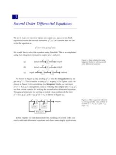
9 Our general solution isthenx(t) =e t[A1exp( 2t) +A2exp( 2t)](17)Figure 1 shows the general forms of the different types of Driven Harmonic OscillatorA common situation is for an Oscillator to be driven by an external force. We will examinethe case for which the external force has a sinusoidal form. The external force can then bewritten asFe=F0cos t, so that the sum of the forces acting on the mass ism x= kx b x+F0cos t(18)We can rearrange this to the form x+ 2 x+ 20x=Acos t(19)where the constants are defined asA F0m, b2m, 0 km(20)4 For the homogeneous solution we have the general solution of a damped Harmonic oscillatorgiven by (11),xh(t) =e t[A1exp( 2 20t) +A2exp( 2 20t)](21)In order to find the particular solution we guess a solution of the formxp(t) =Bcos( t )(this is equivalent toxp(t))

10 =B1cos( t) +B2sin( t) but easier to solve for in this case).Substituting into (19) and expanding the sine and cosine functions we are left with{A B[( 20 2) cos + 2 sin ]}cos t {B[( 20 2) sin 2 cos ]}sin t= 0(22)Since cos tand sin tare linearly independent functions they must vanish to zero for the sin tterm gives ustan =2 20 2(23)From this we arrive atsin =2 ( 20 2)2+ 4 2 2(24)cos = 20 2 ( 20 2)2+ 4 2 2(25)If we now look at the cos tterm from (22) we see thatB=A ( 20 2) cos + 2 sin =A ( 20 2)2+ 4 2 2(26)so that our particular solution isxp(t) =A ( 20 2)