Transcription of The t Distribution and its Applications - Statpower
1 ThetDistribution and its ApplicationsJames H. SteigerDepartment of Psychology and Human DevelopmentVanderbilt UniversityJames H. Steiger (Vanderbilt University)1 / 51 ThetDistribution and its Applications1 Introduction2 Student stDistributionBasic Facts about Student st3 Relationship to the One-SampletDistribution of the Test StatisticThe General Approach to Power CalculationPower Calculation for the 1-SampletSample Size Calculation for the 1-Samplet4 Relationship to thetTest for Two Independent SamplesDistribution of the Test StatisticPower Calculation for the 2-SampletSample Size Calculation for the 2-Samplet5 Relationship to the Correlated SampletDistribution of the Correlated SampletStatistic6 Distribution of the GeneralizedtStatisticSample Size Estimation in the Generalizedt7 Power Analysis via SimulationJames H. Steiger (Vanderbilt University)2 / 51 IntroductionIntroductionIn this module, we review some properties of Student shall then relate these properties to the null and non-nulldistribution of three classic test statistics:1 The 1-Sample Student st-test for a single 2-Sample independent samplet-test for comparing two 2-Sample correlated sample t-test for comparing two meanswith correlated or repeated-measures then discuss power and sample size calculations using thedeveloped H.
2 Steiger (Vanderbilt University)3 / 51 Student stDistributionStudent stDistributionIn a preceding module, we discussed the classicz-statistic for testinga single mean when the population variance is somehow st- Distribution was developed in response to the reality that,unfortunately, 2is not known in the vast majority of substitution of a consistent sample-based estimate of 2(such ass2, the familiar sample variance) will yield a statistic that isstill asymptotically normal, the statistic will no longer have an exactnormal Distribution even when the population Distribution is question of precisely what the Distribution ofY 0 s2/n(1)is when the observations are normal was answered by Student. James H. Steiger (Vanderbilt University)4 / 51 Student stDistributionBasic Facts about Student stStudent stDistributionThe pdf and cdf of thet- Distribution are readily available online atplaces formulae for the functions need not concern us here they arebuilt into key facts, for our purposes, are summarized on the following H.
3 Steiger (Vanderbilt University)5 / 51 Student stDistributionBasic Facts about Student stStudent stDistributionThetdistribution, in its more general form, has two parameters:1 Thedegrees of freedom, 2 Thenoncentrality parameter, When = 0, the Distribution is said to be the central Student st, or simply the tdistribution. When 6= 0, the Distribution is said to be the noncentral Student st, or simply the noncentraltdistribution. The centraltdistribution has a mean of 0 and a variance slightlylarger than the standard normal Distribution . The kurtosis is alsoslightly larger than centraltdistribution is symmetric, while the noncentraltisskewed in the direction of .James H. Steiger (Vanderbilt University)6 / 51 Student stDistributionBasic Facts about Student stStudent stDistributionDistributional CharacterizationIfZis aN(0,1) random variables,Vis a 2 random variable that isindependent ofZand has degrees of freedom, thent , =Z+ V/ (2)has a noncentraltdistribution with degrees of freedom andnoncentrality parameter.
4 James H. Steiger (Vanderbilt University)7 / 51 Relationship to the One-SampletDistribution of the Test StatisticDistribution of the 1-SampletHow does the fundamental result of Equation 2 relate to thedistribution of (Y 0)/ s2/n?First, recall from our Psychology 310 discussion of the chi-squaredistribution thats2 2 2n 1n 1(3)and that, if the observations are taken from a normal Distribution ,thenY ands2are H. Steiger (Vanderbilt University)8 / 51 Relationship to the One-SampletDistribution of the Test StatisticDistribution of the 1-SampletNow let s do some rearranging. Assume that, in this case, =n 0 s2/n=( Y ) + ( 0) 2 2 /(n )=( Y ) 2/n+ n( 0) 2 / (4)We readily recognize that the left term in the numerator is aN(0,1)variable, the right term is = nEs, and the denominator is achi-square divided by its degrees of , sinceY is the only random variable in theZvariate in thenumerator, it is independent of the chi-square variate in , the statistictn 1, =Y 0s/ n(5)must have a noncentraltdistribution withn 1 degrees of freedom,and a noncentrality parameter of = = 0, then = 0 and the statistic has a central H.
5 Steiger (Vanderbilt University)9 / 51 Relationship to the One-SampletThe General Approach to Power CalculationThe General Approach to Power CalculationThe general approach to power calculation is as follows:Under the null hypothesisH0,1 Calculate the Distribution of the test statistic2 Set up rejection regions that establish the probability of a rejection tobe equal to Then specify an alternative state of the world,H1, under which thenull hypothesis is false. UnderH11 Compute the Distribution of the test statistic2 Calculate the probability of obtaining a result that falls in the rejectionregion established H. Steiger (Vanderbilt University)10 / 51 Relationship to the One-SampletThe General Approach to Power CalculationThe General Approach to Power CalculationNote the following key points:Developing expressions for the exact null and non-null distributions ofthe test statistic often requires some specialized statistical general, it is much more likely that expressions for the nulldistribution of the test statistic will be available than expressions forthe non-null , statistical simulation will often provide a reasonablealternative to exact H.
6 Steiger (Vanderbilt University)11 / 51 Relationship to the One-SampletPower Calculation for the 1-SampletPower Calculation for the 1-SampletPower calculation for the 1-Sampletis straightforward if we followthe usual , as with thez-test example, we are pursuing a 1-Samplehypothesis test that specifiesH0: 70 against the alternative thatH1: >70. We will be using a sample ofn= 25 observations, with = the null hypothesis is true, the test statistic will have a centraltdistribution withn 1 = 24 degrees of (one-tailed) critical value will be> qt( , 24)[1] will the power of the test be if = 75 and = 10?James H. Steiger (Vanderbilt University)12 / 51 Relationship to the One-SampletPower Calculation for the 1-SampletPower Calculation for the 1-SampletIn this case, the non-null Distribution is noncentralt, with 24 degreesof freedom, and a noncentrality parameter of nEs= 25(75 70)/10 = power is the probability of exceeding the rejection point in thisnoncentraltdistribution.
7 > 1 - pt(qt( , 24), 24, )[1] gets the identical result, as shown on the next H. Steiger (Vanderbilt University)13 / 51 Relationship to the One-SampletPower Calculation for the 1-SampletPower Calculation for the 1-SampletJames H. Steiger (Vanderbilt University)14 / 51 Relationship to the One-SampletPower Calculation for the 1-SampletPower Calculation for the 1-SampletGPower can do a lot more, including a variety of is one showing power versus sample size whenEs= H. Steiger (Vanderbilt University)15 / 51 Relationship to the One-SampletPower Calculation for the 1-SampletPower Calculation for the 1-SampletOf course, we could generate a similar plot in a few lines of R, andwould then be free to augment the plot in any way we wanted.>### Generic Function for T Rejection Point> <- function(alpha, df, tails){+ if (tails == 2)+ return(qt(1 - alpha/2, df))+ if ((tails^2) !)}
8 = 1)+ return(NA)+ return(tails * qt(1 - alpha, df))+}>### Generic Function for T-Based Power> <- function(delta, df, alpha, tails){+ pow <- NA+ R <- (alpha, df, abs(tails))+ if (tails == 1)+ pow <- 1 - pt(R, df, delta) else if (tails == -1)+ pow <- pt(R, df, delta) else if (tails == 2)+ pow <- pt(-R, df, delta) + 1 - pt(R, df, delta)+ return(pow)+}>### Power Calc for One-Sample T> <- function(mu, mu0, sigma, n, alpha, tails){+ delta = sqrt(n) * (mu - mu0)/sigma+ return( (delta, n - 1, alpha, tails))+}James H. Steiger (Vanderbilt University)16 / 51 Relationship to the One-SampletPower Calculation for the 1-SampletPower Calculation for the 1-Samplet>### Plot Power Curve> curve( (75, 70, 10, x, , 1), 10, 100, xlab = "Sample Size",+ ylab = "Power", col = "red") SizePowerJames H. Steiger (Vanderbilt University)17 / 51 Relationship to the One-SampletSample Size Calculation for the 1-SampletSample Size Calculation for the 1-SampletIn the 1-sampleztest for a single mean, we saw in Psychology 310that it is possible to develop an equation that directly calculates thesample size required to yield a desired level of , in most cases, a closed-form solution fornis not available,because the shape of the test statistic changes along with its locationand spread as a function ofnand the effect , in most cases iterative methods must be methods try an initial value forn, compute an improvementdirection , and step the value ofnin that direction, until thedifference between the computed power and desired power dropsbelow a target modern software, the targetnis found in less than a second formost H.
9 Steiger (Vanderbilt University)18 / 51 Relationship to the One-SampletSample Size Calculation for the 1-SampletSample Size Calculation for the 1-SampletModern power calculation software handles many of the classic casesin parametric statistics. However, in more complex circumstances,remember that, through the use of R s extensive simulation andplotting capabilities, you can obtain power curves and sample-sizecalculations in situations that canned software cannot approach is simple. Plot power versus sample size, then home inon a narrow region of the plot to determine just where sample sizebecomes barely large enough to yield desired H. Steiger (Vanderbilt University)19 / 51 Relationship to the One-SampletSample Size Calculation for the 1-SampletSample Size Calculation for the 1-SampletAn ExampleExample (Sample Size Calculation)Let s try calculating the required sample size to achieve a power whenEs= , and the test is two-sided with = We lluse the graphical approach.
10 Here is a preliminary plot. Notice againthatEscan be input directly by setting 0= 0 and = 1 and setting = a couple of seconds, we have the requirednnarrowed down tobetween 30 and H. Steiger (Vanderbilt University)20 / 51 Relationship to the One-SampletSample Size Calculation for the 1-SampletSample Size Calculation for the 1-SampletAn Example> curve( ( , 0, 1, x, , 2), 10, 100, xlab = "Sample Size",+ ylab = "Power", col = "red")> abline(h = )> abline(v = 30)> abline(v = 35) SizePowerJames H. Steiger (Vanderbilt University)21 / 51 Relationship to the One-SampletSample Size Calculation for the 1-SampletSample Size Calculation for the 1-SampletAn ExampleExample (Sample Size Calculation)Re-plotting the graph with this narrower range and plotting a fewadditional grid lines quickly establishes that the minimum requirednis exact power at this sample size is> ( , 0, 1, 32, , 2)[1] H.