Time series analysis in R - Cornell University

1 Tutorial: Time series analysis in RD G RossiterCornell University , Section of Soil & Crop SciencesISRIC World Soil InformationW 'f0 ffbMarch 14, 2022 Take time to sharpen your axe before you start to chopfirewood. Contents1 Introduction12 Loading and examining a time Example 1: Groundwater level .. Example 2: Daily rainfall .. Answers .. 213 analysis of a single time Summaries .. Numerical summaries .. Graphical summaries .. Smoothing .. Aggregation .. Smoothing by filtering .. Smoothing by local polynomial regression .. Decomposition .. Serial autocorrelation .. Partial autocorrelation .. Spectral analysis .. Answers .. 53 Version Copyright 2009 2012, 2018 2022 D G RossiterAll rights reserved. Reproduction and dissemination of the work as awhole (not parts) freely permitted if this original copyright notice is in-cluded.

2 Sale or placement on a web site where payment must be made toaccess this document is strictly prohibited. To adapt or translate pleasecontact the author Modelling a time Modelling by decomposition .. Modelling by OLS linear regression .. Modelling by GLS linear regression .. Modelling a decomposed series .. Non-parametric tests for trend .. A more difficult example .. Autoregressive integrated moving-average (ARIMA) Autoregressive (AR) models .. Moving average (MA) models .. ARMA models .. ARIMA models .. Periodic autoregressive (PAR) models .. Modelling with ARIMA models .. Checking for stationarity .. Determining the AR degress .. Predicting with ARIMA models .. Answers .. 945 Intervention A known intervention.

3 Answers .. 996 Comparing two time Answers .. 1057 Gap Simulating short gaps in a time series .. Gap filling by interpolation .. Linear interpolation .. Spline interpolation .. Simulating longer gaps in time series .. Non-systematic gaps .. Systematic gaps .. Estimation from other series .. Answers .. 1238 AR models .. Answers .. 129 References130 Index of R concepts132ii1 IntroductionTime series are repeated measurements of one or more variables overtime. They arise in many applications in earth, natural and water re-source studies, including ground and surface water monitoring (qualityand quantity), climate monitoring and modelling, agricultural or otherproduction statistics. Time series have several characteristics that maketheir analysis different from that of non-temporal variables:1.

4 The variable may have atrendover time;2. The variable may exhibit one or morecyclesof different period;3. There will almost always beserial correlationbetween subsequentobservations;4. The variable will almost always have a white noise component, random variation not explained by any of the tutorial presents some aspects of time series analysis (shorthand TSA 1), using theR environment for statistical computing and visu-alisation[12, 14] and its dialect of theS language. R users seriouslyinterested in this topic are well-advised to refer to the text of Metcalfeand Cowpertwait [13]2, part of the excellentUseR! series from Comprehensive R Action Network (CRAN) has a Task View on timeseries analysis4. This lists all the R packages applicable to TSA, catego-rized and with a brief description of each. In addition, Shumway andStoffer [16] is an advanced text which uses R for its examples.

5 Venablesand Ripley [18] include a chapter on time series analysis in S (both R andS-PLUS dialects), mostly using examples from Diggle [8].Good introductions to the concepts of time series analysis are Diggle[8] for biological applications, Box [4] for forecasting and control, Hipeland McLeod [10] (available on the web) for water resources and environ-mental modelling, and Salas [15] from the Handbook of Hydrology forhydrological applications. Davis [7] includes a brief introduction to timeseries for geologists. Wilks [20, Ch. 8] discusses time series for climateanalysis, with emphasis on tutorial is organized as a set oftasksfollowed byquestionsto checkyour understanding;answersare at the end of each section. If you areambitious, there are also some challenges: tasks and questions with nosolution provided, that require the integration of skills learned in to be confused with a bureaucratic monster with the same initials2 Loading and examining a time seriesWe use two datasets5to illustrate different research questions and oper-ations of time series analysis :1.

6 Monthly groundwater levels ( );2. Daily rainfall amounts ( ).These also illustrate some of the problems with importing external datasetsinto R and putting data into a form suitable for time- series the datasets in this exercise are assumed to be stored in theds_tsa datasets subdirectory, under the directory where this tutorial is Example 1: Groundwater levelThe first example dataset is a series of measurements of the depth togroundwater (in meters) in two wells used for irrigation in the Anatolianplateau, Turkey, from January 1975 through December 2004 CE. Theseare provided as text :What are some things that a water manager would want to knowabout this time series ?Jump to A1 Task1: Start R and switch to the directory where the example datasetsare stored. Task2: Examine the file for the first well. You could review the file in a plain-text editor; here we use (".)

7 /ds_ ")Here are the first and last lines of the :Can you tell from this file that it is a time series ?Jump to A2 5kindly provided by colleagues in the University of Twente/faculty ITC s Water Re-sources department, : Read this file into R and examine its structure. Using thescanfunction to read a file into a vector:gw <-scan("./ds_ ")str(gw)## num [1:360] ..Q3:What is the structure?Jump to A3 Task4: Convert the vector of measurements for this well into a timeseries and examine its structure and attributes. Thetsfunction converts a vector into a time series ; it has several argu-ments, of which enough must be given to specify the series : start: starting date of the series ; end: ending date of the series ; frequency: number of observations in the series per unit of time; deltat: fraction of the sampling period between successive one offrequencyordeltatshould be provided, they are two waysto specify the same information.

8 The ending dateendis optional if eitherfrequencyordeltatare given, because the end will just be when thevector this example we know from the metadata that the series begins inJanuary 1975 and ends in December 2004; it is a monthly series . Thesimplest way to specify it is by starting date and the series is established, we examine its structure withstrandattributes <-ts(gw, start=1975, frequency=12)str(gw)## Time- series [1:360] from 1975 to 2005: ..attributes(gw)## $tsp## [1] #### $class## [1] "ts"start(gw)## [1] 1975 1end(gw)## [1] 2004 123In the above example we also show thestartandendfunctions to showthe starting and ending dates in a time : Print the time series ; also show the the time associated witheach measurement, and the position of each observation in the cycle. The genericprintmethod specializes show the actualvalues;timeshows the time associated with each measurement, andcycleshows the position of each observation in the (gw)Here we just show the first and last two Feb Mar Apr May Jun Jul Aug Sep Oct1975 Dec1975 how the month names are automatically assigned.

9 From thetsdoc-umentation: Values of 4 and 12 are assumed in print methods to imply aquarterly and monthly series respectively. (gw)Again, only the beginning and end of the full series :Jan Feb Mar Apr May Jun Jul1975 Sep Oct Nov Dec1975 (gw)Again, only the beginning and end of the full series :Jan Feb Mar Apr May Jun Jul Aug Sep Oct Nov Dec1975 1 2 3 4 5 6 7 8 9 10 11 121976 1 2 3 4 5 6 7 8 9 10 11 1 2 3 4 5 6 7 8 9 10 11 122004 1 2 3 4 5 6 7 8 9 10 11 124Q4:What are the units of each of these?Jump to A4 Task6: Determine the series frequency and interval between observa-tions. Of course we know this from the metadata, but this information canalso be extracted from the series object with thefrequencyanddeltat,methods, as in the arguments (gw)## [1] 12deltat(gw)## [1] :What are the units of each of these?

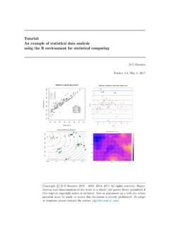
10 Jump to A5 Task7: Plot the time series . The genericplotmethod specializes time- series are several ways to visualise this, we show a few possibilities here:par(mfrow=c(1,3))# pdf(" ", width=10, height=5)plot(gw, ylab="Depth to water table (m)", main="Anatolia Well 1")# ()plot(gw, type="o", pch=20, cex= , col="blue",ylab="Depth to water table (m)", main="Anatolia Well 1")plot(gw, type="h", col="blue", ylab="Depth to water table (m)",main="Anatolia Well 1")par(mfrow=c(1,1))Anatolia Well 1 TimeDepth to water table (m)1975198019851990199520002005303540455 055 Anatolia Well 1 TimeDepth to water table (m)1975198019851990199520002005303540455 055 Anatolia Well 1 TimeDepth to water table (m)1975198019851990199520002005303540455 055Q6:What are the outstanding features of this time series ? Jump to A6 5 Task8: Plot three cycles of the time series , from the shallowest depthat the end of the winter rains (April) beginning in 1990, to see annualbehaviour.