Transcription of Topic 3 The -function & convolution. Impulse response ...
1 Topic 3 The -function & response & Transfer functionIn this lecture we will described the mathematic operation of theconvolutionoftwo continuous functions . As the name suggests, two functions are blended orfolded will then discuss theimpulse responseof a system, and show how it is relatedto the transfer function of the though we will define a special function called the -function or unit is, like the Heaviside step functionu(t), a generalized function or distribution and is best defined by considering another function in conjunction with The -functionConsider a functiong(t) ={1/w0< t < w0otherwiseOne thing of note aboutg(t) is that w0 g(t)dt= lower limit 0 is a infinitesimally small amount less than zero. Now, supposethat the widthwgets very small, indeed as small at 0+, an number an infinitesimalamount bigger than zero.}
2 At that point,g(t) has become like the function, avery thin, very high spike at zero, such that (t)dt= 0+0 (t)dt= 113/2w1/w0g(t)0(t) (a)(b)Figure : Aswbecomes very small the functiong(t) turns into a -function (t) indicated bythe arrowed some sense it is akin to the derivative of the Heaviside unit step t (t)dt=u(t).More formally the delta function is defined in association with any arbitrary functionf(t), asThe delta function .. f(t) (t)dt=f(0).Picking out values of a function in this way is calledsiftingoff(t) by (t). Wecan also see that f(t) (t )dt=f( ),a result that we will return (t)f(t)0f(t) (t ) t (t )0 tA(a)(b)(c)Figure : (a,b) Sifting. (c) With an the -function is infinitely high, very often you will see a described asthe unit -function, or see a -function spike with an amplitudeAby it.
3 This is todenote a delta -function where (t)dt= 1 or A (t)dt= Properties of the -functionFourier transform of the delta function:FT[ (t)] = 1 Proof:Use the definition of the -function and sift the functionf(t) = e i t: (t)e i tdt= e i 0= :The -function has even symmetry. (t) = ( t)Parameter Scaling: (at) =1|a| (t)Proof:To prove this return to the fundamental definition, f(t) (t)dt=f(0)Ifa 0, substitute (at) fort(no swap in limits) f(at) (at)d(at)=a f(at) (at)dt=f(0)But f(at) (t)dt=f(0) a (at) = (t).Now ifa <0, substitute (at) fort(but need to swap limits asanegative) f(at) (at)d(at)= a f(at) (at)dt=f(0)But f(at) (t)dt=f(0) a (at) = (t).So|a| (at) = (t) covers both cases, and the stated definition follows Fourier Transforms that involve the -functionFourier Transform ofei 0tFT[ei 0t]= ei( 0 )tdt= 2 ( 0).
4 Fourier Transform of1FT[1] = 2 ( ).You could obtain this either by putting 0= 0 just above, or by using the dualproperty,FT[1] = 2 ( ), then the even symmetry property ( ) = ( ).Fourier Transform ofcos 0tFT[cos 0t] =FT[12(ei 0t+ e i 0t)]= ( ( 0) + ( + 0)).Fourier Transform ofsin 0tFT[cos 0t] =FT[12i(ei 0t e i 0t)]= i ( ( 0) ( + 0)).Fourier Transform of Complex Fourier Series yes, this can be useful!FT[n= n= Cnein 0t]= 2 n= n= Cn ( n 0). ConvolutionWe turn now to a very important technique is signal analysis and processing. Theconvolution of two functionsf(t) andg(t) is denoted byf g. The convolutionis defined by an integral over the dummy variable .The convolution value off gattis(f g)(t) = f( )g(t )d 3/5 The process is commutative, which means that(f g)(t) (g f)(t)or f( )g(t )d f(t )g( )d Example 1It is easier to see what is going on when convolving a signalfwith a functiongof even or odd symmetry.
5 However, to get into a strict routine, it is best to startwith an example with no symmetry.[Q]Find and sketch the convolution off(t) =u(t)e atwithg(t) =u(t)e bt,where bothaandbare positive.[A]Using the first form of the convolution integral, the short answer must bethe unintelligiblef g= u( )e a u(t )e b(t )d .First, make sketches of the functionsf( ) andg(t ) as varies. Functionf( )looks just likef(t) of course. Butg(t ) is a reflected ( time reversed ) andshifted version ofg(t). (The reflection is easy enough. To check that the shiftis correct, ask yourself where does the functiong(p) drop? The answer is atp= 0. Sog(t ) must drop whent = 0, that is when =t.)0 f( )) g(0 )g( 0 0 g(t )t(a)(b) (c) (d)Figure :We now multiply the two functions , BUT we must worry about the fact thattisa variable.
6 In this case there are two different regimes, one whent <0 and theother whent 0. Figure shows the now to the integration. Fort <0, the function on the bottom left of is everywhere zero, and the result is zero. Fort 0 u( )e a u(t )e b(t )d =e bt t0e(b a) d =e btb a(e(b a)t 1)3/6f( )g(t )0 g(t )f() tt0t<0f( )g(t )0 tg(t )f() t>0t0 Figure :Sof g(t) ={(e at e bt)/(b a) fort 00fort <0It is important to realize that the function at the bottom right of Figure isNOT the convolution. That is the function you are about to integrate over for aparticular value oft. Figure shows thet >0 part of the convolution forb= 2anda= 1. 0 0 1 2 3 4 5 6(exp(-x)-exp(-2*x))Figure :f g(t) plotted fort >0 whenb= 2 anda= Example 2[Q]Derive an expression for the convolution of an arbitrary signalf(t) with thefunctiong(t) shown in the figure.}
7 Determine the convolution whenf(t) =A, aconstant, and whenf(t) =A+ (B A)u(t).[A]Follow the routine. Functionf( ) looks exactly likef(t), butg(t ) isreflected and shifted. Multiply and integrate over from to . Becausegonly has finite range, we can pinch in the limits of integration, and the convolutionbecomesf g= tt af( )d + t+atf( )d f(t)tg(t)ta a1 1g(t )f(t)t1 1t+at a tFigure :Whenf(t) =A, a constant, it is obvious by inspection that the convolution is zerofor allt. Whenf(t) =A+ (B A)u(t), we have to be more careful becausethere is a discontinuity in the Figure (a): The convolution is zero for allt < aand allt > a(Diagram positions1,2,5). The maximum value is whent= 0 (Position 4). By inspection, or using theintegrals above, (f g)(t= 0) =a(B A).
8 For a < t <0, (Position 3)f g= tt a(A)d + 0tAd + t+a0Bd = aA+ tA+(t+a)B= (a+t)(B A)showing that the increase in correlation value is linear. Symmetry tells us thatthe decrease for 0< t < awill also be can see from Figure (b) that this convolution provides a rudimentary de-tector of steps in the signal. The maximum in the correlation is proportion to thestep size, and would go negative if the step was (t )4:t=0f( )f( )g(t )ABa a a 2a0001:2:t= a a<t<03:5:t>a t< af*gta aa(B A)(a)(b)Figure The Impulse response FunctionYou are very used to describing systems using the transfer function in the frequencydomain. So used to it in fact, that you may have forgotten to wonderwhy can twe describe a system s response in the time domain?The answer isYou can, butyou didn t know about convolution until the time domain, a system is described by itsImpulse response Functionh(t).
9 This function literally describes the response of system at timetto an unitimpulse or -function input administered at timet= that now is timet, and you administered an Impulse to the system attime in the past. The response now isy(t) =h(t ).t0 NowtWhacktx(t)Succession of whacks Figure :Suppose you administered a succession of impulses of different strengthsx. Theportion dy(t) of the response due to Impulse a time earlier isdy(t) =x( )h(t )d ,so that the total response now isy(t) = t x( )h(t )d ,where all suppose thathiscausal. If > tthenh(t ) = 0, and therefore,providedh(t)is causal,the time responsey(t)to an inputx(t)isy(t)= x( )h(t )d =x h .The output is the input CONVOLVED with the Impulse How do we connect this up ..Can we reconcile the following things you now know about systems and signals?
10 Temporal output is the temporal input CONVOLVED with the ImpulseResponse frequency domain output is the frequency domain input MULTIPLIEDby the Transfer frequency domain signal is the Fourier Transform of the temporal signalMathematically, it must be that the FT of a convolution is a (t) =x(t) h(t) FTFT ? ?Y( ) =X( )H( ) The Fourier Transform of a ConvolutionTo prove this we need to develop the integration for the Fourier Transform of aconvolution. Nowx his a perfectly respectable function oft, soFT[x h] = t= [(x h)(t)] e i tdt= t= = x( )h(t )d e i tdt3/10 For absolute clarity, let s switch the order of integration, then writet= +p. Inthe inner integral is a constant, so that dt= [x h] = = t= x( )h(t )e i tdtd = = p= x( )h(p)e i e i pdpd = = x( )e i d p= h(p)e i pdp=FT[x]FT[h]=X( )H( )So, the first important thing we discover isThe time-convolution/frequency-modulation property of Fouriertransformf(t) g(t) F( )G( )orFT[f(t) g(t)] =FT[f(t)]FT[g(t)] =F( )G( ) Impulse response and Transfer FunctionThe second important connection is thatThe Fourier Transform of the Impulse response Function is the Trans-fer Functionh(t) H( )orFT[h(t)] =H( )3/11*h(t)x(t)y(t)X( Y()) )H(Figure The time-modulation/frequency-convolution propertyThere is a further result involving convolution that we state modulation/convolution property of Fourier transformf(t)g(t) 12 F( ) G( )