Transcription of Topological Data Analysis - arXiv
1 Topological data Analysis Larry Wasserman Department of Statistics/Carnegie Mellon University Pittsburgh, USA, 15217; email: Abstract Topological data Analysis (TDA) can broadly be described as a collec- [ ] 27 Sep 2016. tion of data Analysis methods that find structure in data . This includes: clustering, manifold estimation, nonlinear dimension reduction, mode es- timation, ridge estimation and persistent homology. This paper reviews some of these methods. Contents 1 INTRODUCTION 2. 2 DENSITY CLUSTERS 2. Level Set Clusters .. 2. Density Trees .. 4. Mode Clustering and Morse Theory .. 7. 3 LOW DIMENSIONAL SUBSETS 9. Manifolds .. 9. Estimating Intrinsic Dimension .. 13. Ridges .. 13.
2 Stratified Spaces .. 16. 4 PERSISTENT HOMOLOGY 16. Homology .. 17. Distance Functions and Persistent Homology .. 18. Simplicial Complexes .. 21. Back To Density Clustering .. 23. 5 TUNING PARAMETERS AND LOSS FUNCTIONS 24. 6 data VISUALIZATION AND EMBEDDINGS 27. 7 APPLICATIONS 28. The Cosmic Web .. 28. Images .. 29. Proteins .. 29. Other Applications .. 31. 8 CONCLUSION: THE FUTURE OF TDA 32. 1. 1 INTRODUCTION. Topological data Analysis (TDA) refers to statistical methods that find struc- ture in data . As the name suggests, these methods make use of Topological ideas. Often, the term TDA is used narrowly to describe a particular method called persistent homology (discussed in Section 4).
3 In this review, I take a broader perspective: I use the term TDA to refer to a large class of data anal- ysis method that uses notions of shape and connectivity. The advantage of taking this broader definition of TDA is that it provides more context for re- cently developed methods. The disadvantage is that my review must necessarily be incomplete. In particular, I omit any reference to classical notions of shape such as shape manifolds (Kendall, 1984; Patrangenaru & Ellingson, 2015) and related ideas. Clustering is the simplest example of TDA. Clustering is a huge topic and I. will only discuss density clustering since this connects clustering to other meth- ods in TDA. I will also selectively review aspects of manifold estimation (also called manifold learning ), nonlinear dimension reduction, mode and ridge es- timation and persistent homology.
4 In my view, the main purpose of TDA is to help the data analyst summarize and visualize complex datasets. Whether or not TDA can be used to make scientific discoveries is still unclear. There is another field that deals with the Topological and geometric structure of data : computational geometry. The main difference is that in TDA we treat the data as random points whereas in computational geometry the data are usually seen as fixed. Throughout this paper, we assume that we observe a sample X1 , .. , Xn P (1). where the distribution P is supported on some set X Rd . Some of the technical results cited require either that P have sufficiently thin tails or that X be compact. Software: many of the methods in this paper are implemented in the R.
5 Package TDA available at A tutorial on the package can be found in Fasy et al. (2014a). 2 DENSITY CLUSTERS. Clustering is perhaps the oldest and simplest version of TDA. The connection between clustering and topology is clearest if we focus on density-based methods for clustering. Level Set Clusters Let X1 , .. , Xn be a random sample from a distribution P with density p where Xi X Rd . Density clusters are sets with high density. Hartigan (1975, 2. 1981) formalized this as follows. For any t 0 define the upper level set n o Lt = x : p(x) > t . (2). The density clusters at level t, denoted by Ct , are the connected components of Lt . The set of all density clusters is [. C= Ct . (3).]
6 T 0. The leftmost plot in Figure 1 shows a density function. The middle plot shows the level set clusters corresponding to one particular value of t. The estimated upper level set is n o L. b t = x : pb(x) > t (4). where pb is any density estimator. A common choice is the kernel density esti- mator n . 1X 1 ||x Xi ||. pbh (x) = K (5). n i=1 hd h where h > 0 is the bandwidth and K is the kernel. The theoretical properties of the estimator L b t are discussed, for example, in Cadre (2006) and Rinaldo &. Wasserman (2010). In particular, Cadre (2006) shows, under regularity condi- tions and appropriate h, that (L b t Lt ) = OP (1/ nhd ) where is Lebesgue measure and A B is the set difference between two sets A and B.
7 To find the clusters, we need to get the connected components of L b t . Let It = {i : pbh (Xi ) > t}. Create a graph whose nodes correspond to (Xi : i It ). Put an edge between two nodes Xi and Xj if ||Xi Xj || where > 0. is a tuning parameter. (In practice = 2h often seems to work well.) The connected conponenets C b1 , C. b2 , .. of the graph estimate the clusters at level t. The number of connected components is denoted by 0 which is the zeroth-order Betti number. This is discussed in more detail in Section Related to level sets is the concept of excess mass. Given a class of sets C, the excess mass functional is defined to be E(t) = sup{P (C) t (C) : C C} (6). and any set C C such that P (C) t (C) = E(t) is called a generalized t- cluster.
8 If C is taken to be all measurable sets and the density is bounded and continous, then the upper level set Lt is the unique t-cluster. The excess mass functional is studied in Polonik (1995); Mu ller & Sawitzki (1991). One question that arises in the use of level set clustering is: how do we choose t? One possibility is to choose t to cover R some prescribed fraction 1 . of the total mass; thus we choose t to satisfy Lbt pb(s)ds = 1 . Another idea is to look at clusters at all levels t. This leads us to the idea of density trees. 3. t Figure 1: Left: a density function p. Middle: density clusters corresponding to Lt = {x : p(x) > t}. Right: the density tree corresponding to p is shown under the density.
9 The leaves of the tree correspond to modes. The branches correspond to connected components of the level sets. Density Trees The set of all density clusters T C has a tree structure: if A, B C then either A B or B A or A B = . For this reason, we can visually represent a density and its clusters as a tree which we denote by Tp or T (p). Note that Tp is technically a collection of level sets, but it can be represented as a two- dimensional tree as in the right-most plot in Figure 1. The tree, shown under the density function, shows the number of level sets and shows when level sets merge. For example, if we cut across at some level t, then the number of braches of the tree corresponds to the number of connected components of the level set.
10 The leaves of the tree correspond to the modes of the density. The tree is called a density tree or cluster tree. This tree provides a conve- nient, two-dimensional visualization of a density regardless of the dimension d of the space in which the data lie. Two density trees have the same shape if their tree structure is the same. Chen et al. (2016) make this precise as follows. For a given tree Tp define a distance on the tree by dTp (x, y) = |p(x) + p(y) 2mp (x, y)|. where mp (x, y) = sup{t : there exists C Ct such that x, y C}. is called the merge height (Eldridge et al., 2015). For any two clusters C1 , C2 . Tp , we first define 1 = sup{t : C1 Ct }, and 2 analogously. We then define the tree distance function on Tp by dTp (C1 , C2 ) = 1 + 2 2mp (C1 , C2 ) (7).
![arXiv:0706.3639v1 [cs.AI] 25 Jun 2007](/cache/preview/4/1/3/9/3/1/4/b/thumb-4139314b93ef86b7b4c2d05ebcc88e46.jpg)
![arXiv:1301.3781v3 [cs.CL] 7 Sep 2013](/cache/preview/4/d/5/0/4/3/4/0/thumb-4d504340120163c0bdf3f4678d8d217f.jpg)
![@google.com arXiv:1609.03499v2 [cs.SD] 19 Sep 2016](/cache/preview/c/3/4/9/4/6/9/b/thumb-c349469b499107d21e221f2ac908f8b2.jpg)