Transcription of Transmission line T - Spice Model
1 Analog devicesT222 Transmission lineDescriptionThe Transmission line device is a bidirectional delay line with two ports, A and B. The (+) and (-) nodes define the polarity of a positive voltage at a transient (.TRAN (transient analysis)) analysis, the internal time step is limited to be no more than one-half the smallest Transmission delay, so short Transmission lines cause long run simulation status window displays the properties of the three shortest Transmission lines in a circuit if a transient run s time step ceiling is set more frequently by one of the Transmission lines. This is helpful when you have a large number of Transmission lines. The properties displayed are: % loss: percent attenuation at the characteristic delay ( , the degree to which the line is lossy) time step ceiling: induced by the line % of line delay: time step size at percentage of characteristic delayThese Transmission line properties are displayed only if they are slowing down the a line that uses a Model , the electrical length is given after the Model name.
2 Example T5 of Examples uses TMOD to specify the line parameters and has an electrical length of one unit. All of the Transmission line parameters from either the ideal or lossy parameter set can be expressions. In addition, R and G can be general Laplace expressions. This allows the user to Model frequency dependent effects, such as skin effect and dielectric loss. However, this adds to the computation time for transient analysis, since the impulse responses must be obtained by an inverse FFT instead of devicesTIdeal line General formT<name> <A port (+) node> <A port (-) node>+ <B port (+) node> <B port (-) node>+ [ Model name]+ Z0=<value> [TD=<value>] [F=<value> [NL=<value>]]+ IC= <near voltage> <near current> <far voltage> <far current>Description As shown below, port A s (+) and (-) nodes are 1 and 2, and port B s (+) and (-) nodes are 3 and 4, the ideal line , IC sets the initial guess for the voltage or current across the ports.
3 The <near voltage> value is the voltage across A(+) and A(-) and the <far voltage> is the voltage across B(+) and B(-). The <near current> is the current through A(+) and A(-) and the <far current> is the current through B(+) and B(-).For the ideal case, Z0 is the characteristic impedance. The Transmission line s length can be specified either by TD, a delay in seconds, or by F and NL, a frequency and a relative wavelength at F. NL has a default value of (F is the quarter-wave frequency). Although TD and F are both shown as optional, one of the two must be Z0 (Z-zero) and ZO (Z-O) are accepted by the 13delayed V3 V4Z0Z0I12-I34delayed I1delayed V1 V2 Analog devicesT224 Lossy line General formT<name> <A port (+) node> <A port (-) node>+ <B port (+) node> <B port (-) node>+ [ < Model name> [electrical length value] ]+ LEN=<value> R=<value> L=<value>+ G=<value> C=<value>ExamplesT1 1 2 3 4 Z0=220 TD=115nsT2 1 2 3 4 Z0=220 F= 1 2 3 4 Z0=220 F= NL= 1 2 3 4 LEN=1 R=.
4 311 L=.378u G= C= 1 2 3 4 TMOD 1 Model < Model name> TRN [ Model parameters]DescriptionThe simulator uses a distributed Model to represent the properties of a lossy Transmission line . That is, the line resistance, inductance, conductance, and capacitance are all continuously apportioned along the line s length. A common approach to simulating lossy lines is to Model these characteristics using discrete passive elements to represent small sections of the line . This is the lumped Model approach, and it involves connecting a set of many small subcircuits in series as shown below:This method requires that there is enough lumps to adequately represent the distributed character of the line , and this often results in the need for a large netlist and correspondingly long simulation times. The method also produces spurious oscillations near the natural frequencies of the lumped additional extension allows systems of coupled Transmission lines to be simulated.
5 Transmission line coupling is specified using the K device. This is done in much the same way that coupling is specified for inductors. See the description of Transmission line coupling for further distributed Model allows freedom from having to determine how many lumps are sufficient, and eliminates the spurious oscillations. It also allows lossy lines to be simulated in a fraction of the time necessary when using the lumped approach, for the same a lossy line , LEN is the electrical length. R, L, G, and C are the per unit length values of resistance, inductance, conductance, and capacitance, respectively. Example T4 specifies a lossy line one meter long. The lossy line Model is similar to that of the ideal case, except that the delayed voltage and current values include terms which vary with frequency. These terms are computed in transient analysis using an impulse response convolution method, and the internal time step is limited by the time resolution required to accurately Model the frequency characteristics of the line .
6 As with ideal lines, short lossy lines cause long run line segmentRLGC225 Analog devicesTCapture partsIdeal and lossy Transmission linesListed below are the properties that you can set per instance of an ideal (T) or lossy (TLOSSY) Transmission line . The parts contained in the part library contain a variety of Transmission line types. Their part properties A/D uses a distributed Model to represent the properties of a lossy Transmission line . That is, the line resistance, inductance, conductance, and capacitance are all continuously apportioned along the line s common approach to simulating lossy lines is to Model these characteristics using discreet passive elements to represent small sections of the line . This is the lumped Model approach, and it involves connecting a set of many small subcircuits in series. This method requires that enough lumps exist to adequately represent the distributed characteristic of the line .
7 This often results in the need for a large netlist and correspondingly long simulation time. The method also produces spurious oscillations near the natural frequencies of the lumped distributed Model used in PSpice A/D frees you from having to determine how many lumps are sufficient, and eliminates the spurious oscillations. It also allows lossy lines to be simulated with the same accuracy in a fraction of the time required by the lumped addition, you can make R and G general Laplace expressions. This allows frequency dependent effects to be modeled, such as skin effect and dielectric nameModel typeProperty Property descriptionTtransmission lineZ0characteristic impedanceTDtransmission delayFfrequency for NLNL number of wavelengths or wave numberTLOSSY**Not available for Basics+ lineLENelectrical lengthRper unit length resistanceLper unit length inductanceGper unit length conductanceCper unit length capacitanceAnalog devicesT226 Coupled Transmission linesListed below are the properties that you can set per instance of a coupled Transmission line part.
8 The part library provides parts that can accommodate up to five coupled Transmission lines. You can also create new parts that have up to ten coupled nameModel typeProperty Property descriptionT2 COUPLEDT3 COUPLEDT4 COUPLEDT5 COUPLED coupled Transmission line symmetricLENelectrical lengthRper unit length resistanceLper unit length inductanceGper unit length conductanceT2 COUPLEDX*T3 COUPLEDXT4 COUPLEDXT5 COUPLEDX*T2 COUPLEDX is functionally identical to T2 COUPLED. However, the T2 COUPLEDX implementation uses the expansion of the subcircuit referenced by Transmission line asymmetricLENelectrical lengthRper unit length resistanceLper unit length inductanceGper unit length conductanceCper unit length capacitanceLMper unit length mutual inductanceCMper unit length mutual capacitanceKCOUPLE2transmission line coupling matrix T1name of first coupled lineT2name of second coupled lineLMper unit length mutual inductanceCMper unit length mutual capacitanceKCOUPLE3 KCOUPLE4 KCOUPLE5T1name of first coupled lineT2name of second coupled lineT3name of third coupled lineLMijper unit length mutual inductance between line Ti and line TjCMijper unit length mutual capacitance between line Ti and line Tj227 Analog devicesTSimulating coupled linesUse the K device to simulate coupling between Transmission lines.
9 Each of the coupled Transmission line parts provided in the standard part library translate to K device and T device declarations in the netlist. PSpice A/D compiles a system of coupled lines by assembling capacitive and inductive coupling matrices from all of the K devices involving Transmission lines. Though the maximum order for any one system is ten lines, there is no explicit limitation on the number of separate systems that may appear in one simulation. The simulation Model is accurate for: ideal lines low-loss lossy lines systems of homogeneous, equally spaced high-loss linesFor more information, see Transmission line considerationsWhen simulating, Transmission lines with short delays can create performance bottlenecks by setting the time step ceiling to a very small one Transmission line sets the time step ceiling frequently, PSpice A/D reports the three lines with the shortest time step. The status window displays the percentage attenuation, step ceiling, and step ceiling as percentage of Transmission line your simulation is running reasonably fast, you can ignore this information and let the simulation proceed.
10 If the simulation is slowed significantly, you may want to cancel the simulation and modify your design. If the line is lossy and shows negligible attenuation, Model the line as ideal devicesT228 Transmission line Model parametersModel parameters** ( Model definition). The order is from the most commonly used to the least commonly used ** Any length units can be used, but they must be consistent. For instance, if LEN is in feet, then the units of R must be in ohms/foot.** A lossy line with R=G=0 and LEN=1 is equivalent to an ideal line with and .Defaultfor all Transmission linesIC Sets the initial condition and all four values must be entered. Four values are expected when IC is specified: the near-end voltage, the near-end current, the far-end voltage, and the far-end current, given in that ideal Transmission linesZO characteristic impedanceohmsnoneTD Transmission delaysecondsnoneF frequency for NLHznoneNL relative lossy Transmission linesR per unit length resistanceohms/unit lengthnoneL per unit length inductancehenries/unit lengthnoneG per unit length conductancemhos/unit lengthnoneC per unit length capacitancefarads/unit lengthnoneLEN** physical lengthagrees with RLGC *noneZOLC---=TDLENL C =229 Analog devicesTReferences For more information on how the lossy Transmission line is implemented, refer to:[1] Roychowdhury and Pederson, Efficient Transient Simulation of Lossy Interconnect, Design Automation Conference, 1991.
