Transcription of Transmission Lines at Audio Frequencies, and a Bit …
1 Transmission Lines at Audio frequencies , and a Bit of History by Jim Brown Audio Systems Group, Inc. Entire contents 2005-2008 The Audio Systems Group, Inc. All rights reserved. If you study Transmission Lines in college or from the ARRL Handbook, you will learn the clas-sic equation for characteristic impedance. ZO = [ L/C) ]1/2 What most of us have long forgotten (and that few universities teach) is that this is the simpli-fied form of the equation. In engineering classes, we make equations simpler by assuming certain conditions will be true for what we think will be the conditions when we use them. That s fine as long as we don t forget those assumption, but in this case, most of us have. The full equation for characteristic impedance is ZO = [ (R+j2 fL) / (G+j2 fC) ]1/2 At high frequencies (that is, f is large), (2 fL) is much larger than R, and (2 fC) is much larger than G.
2 So at high frequencies , the equation becomes simply ZO = [ j2 fL) / j2 fC) ]1/2 and further simplifies to ZO = [ L/C) ]1/2 which is the familiar equation. But what if f is not large? Fig 1 shows the impedance of a typi-cal coaxial cable at Audio frequencies using the full equation. Why the wide variation? Be-cause at low frequencies , R is much greater than 2 fL, and 2 fC is much greater than G. Thus, at low Audio frequencies , the equation simplifies to ZO = [R/j2 fC]1/2. Within the Audio spectrum and for a decade or so above it, R in this equation is simply the DC resistance of the cable(per the same unit length as the L and C parameters). This causes the impedance to be quite high and predominantly capacitive near zero frequency. As frequency increases, L becomes significant, and ZO transitions to the familiar 50-100 ohm impedances at high fre-quencies.
3 And the transition occurs right in the middle of the Audio spectrum! Through the transition region, the "j" term causes ZO to be a combination of resistance and capacitance. [Although the data presented here is for coaxial cables, virtually all commonly used cables, including twisted pairs, exhibit these characteristics!] Above the Audio spectrum, R begins to increase with skin effect as the square root of frequency, causing attenuation to increase. Fig. 1 Characteristic Impedance of Typical Cable at Audio frequencies [6] Fig. 2 Velocity of Propagation of Typical Cable at Audio frequencies [6] The graph for velocity of propagation (Fig 2) yields a similar surprise, going through the same sort of transition, and for the same reason. These data are computed for the theoretical case of a line terminated in its characteristic impedance, which, as we have just learned, varies over two orders of magnitude.
4 Indeed, all of the characteristics of a cable vary by nearly two orders of magnitude through the Audio spectrum the lowest frequencies take 50 times longer to get to the other end of the cable than the high frequencies ! These effects are too Cable, Transmission Lines , and Shielding for Audio and Video Systems Page 2 small to notice in a theater where cables are rarely more than 500 ft long, but they can be quite significant on a telephone line that is tens of miles long! So we see that the behavior of Transmission Lines at low frequencies is, indeed, a very com-plex matter. Telegraph and telephone companies learned early on that very long Lines (tens and hundreds of miles) need to be equalized both for frequency response and to maintain velocity of propagation reasonably constant. Without that equalization, they could not even transmit Morse Code reliably on long circuits.
5 Later, on the first transcontinental telephone circuits, voices were mangled beyond recognition. In both cases, the cause was the variation in VP over the Audio spectrum. In 1893, the physicist Oliver Heavyside showed that if R/L could be made equal to G/C (or RC=GL), a constant velocity of propagation would result and the attenuation would be mini-mized. The problem was (and is) that in practical cables, L is much too small to achieve these ratios. In the earliest days of the telegraph (the latter half of the 19th century), the signal was carried on a single iron wire strung on poles with the earth as a return. These circuits had more L, both because of their spacing and the use of the iron wire, and the variation in veloc-ity was not too much of a problem for telegraphy (in those days, there was no AC power to induce hum). With the advent of the telephone (invented in the late 1870's), many more cir-cuits and greater bandwidth without time distortion was needed To provide more circuits and reduce crosstalk, twisted pair copper cables were developed.
6 This made L (the loop in-ductance) much smaller, which in combination with the Transmission of Audio motivated Heavyside's thinking. The modern solution, based on Heavyside's work, developed by M. I. Pupin and G. A. Campbell, and patented by Pupin in 1900, was (and still is) to add inductors in series with a long line at intervals of several thousand feet. This serves to turn the line into a bandpass filter with a sharp cutoff between 3 kHz and 15 kHz, depending on how large the inductors are and how closely the inductors were spaced. Ordinary telephone voice circuits are equalized using 88 mH inductors at intervals of about 6,000 ft, resulting in an upper cutoff frequency of 3 kHz. Greater bandwidth could be achieved with smaller inductors and/or shorter spacing, and with the addition of repeater amplifiers along the way. The addition of the inductors did four important things it extended the frequency response, it equalized the delay, it made the impedance more constant, and it imposed the low-pass filter characteristic.
7 Eventually the repeaters themselves were designed to provide equalization. The work that made these equalizing repeaters possible was done by Harold Black (the inventor of negative feedback), Harry Nyquist, and Hendrik Bode, all of them engineers at Bell Labs! [3] If cables could be constructed with the desired R, L, G, and C relationships for constant ve-locity of propagation, they would not have that extreme low pass characteristic. It is the addi-tion of the discrete inductors that does that! Loading can be done continuously, and even the earliest transoceanic cables were continuously loaded. [1] To provide continuous loading, the center conductor of the more modern of these cables were wrapped with permalloy tape having a high permeability. This provided equalization of both time and amplitude response, but without the low pass filter. Around 1960, for example, one such trans-Atlantic cables op-erated as a carrier-based system (that is, Audio was modulated onto radio carriers and sent over the cable), and was carrying 36 high grade circuits plus some utility grade circuits, and was planning an expansion to 48 circuits.
8 Although the bandwidth of this cable or the circuits is not stated in the reference, the number of circuits implies bandwidth of at least several hundred kHz. [2] Note also that such cables will still exhibit the more gentle low pass char-acteristic due losses that increase with frequency (mostly due to skin effect). Myth 600 ohms and open wire line . Calvert computes Zo, Vp and attenuation for an open wire line that was commonly used in early telephony-- #12 AWG copper spaced 12" apart, and for which the basic parameters were well documented. For dry weather, G = S/mile, R = /mile, L = mH/mile, and C = nF/mile. At 300 Hz, ZO is 1,345 , VP = m/s (VF= ); at 1,000 Hz, ZO = 841 , VP = m/s (VF= ); and at 3 kHz, ZO = 712 , VP = m/s (VF= ). Attenuation is Cable, Transmission Lines , and Shielding for Audio and Video Systems Page 3 dB/mile at 300 Hz, dB/mile at 1 kHz, and dB/mile at 3 kHz.
9 Fundamental Cable Parameters can be computed from manufacturers' data. ZO at radio frequencies is published for most cables. So are resistance and capacitance per unit length. The inductance per unit length is simply C ZO2. For coax, C ranges between 20 and 32 pF/ft, L between H/ft and H/ft. RDC ranges between 2 and 50 m /ft. For balanced Audio cables, C ranges between 12 and 40 pF/ft (as high as 110 pF/ft for star quad cables); ZO at radio frequencies is on the order of 60-90 ohms (110 ohms for digital cables), L is about H/ft, and R is typically 20-50 m /ft. Finding the value of R at radio frequencies in m /ft is significantly more difficult. Witt [7, 8] published a Mathcad worksheet that iteratively computes these values from manufacturers data for attenuation vs frequency. His model uses the complex form of the equations for ZO and attenuation, and assumes that skin effect causes R to increase with the square root of frequency.
10 From this, he concludes that in coaxial cables, resistive loss in the conductors is the dominant component of cable loss to at least 1 GHz, and that dielectric loss becomes significant and then dominates above about 2 GHz. Comparable work for balanced Audio cables is likely to yield similar results. Electrical Wavelength at Audio Fre-quencies can be computed from Fig 2. At 1/20 wavelength and below, trans-mission line effects are negligible, and the circuit can be analyzed using simple lumped circuit parameters. At 1/10 wavelength, Transmission line effects are still quite small, and can generally be neglected. Fig 3 shows the characteris-tics of the RG59 cable of Fig 2. Typical balanced Audio cables have similar properties, typically differing from Fig 1, 2, and 3 by no more than a factor of 2 in frequency.