Transcription of Two-way (between-groups) ANOVA in R
1 Two-way ANOVA in R statstutor Community Project Sofia Maria Karadimitriou and Ellen Marshall University of Sheffield stcp-karadimitriou-ANOVA2 Two-way ( between -groups) ANOVA in R Dependent variable: Continuous (scale/interval/ratio), Independent variables: Two categorical (grouping factors) Common Applications: Comparing means for combinations of two independent categorical variables (factors). Data: The data set contains information on 78 people who undertook one of three diets. There is background information such as age, gender (Female=0, Male=1) and height. The aim of the study was to see which diet was best for losing weight but it was also thought that the best diets for males and females may be different so the independent variables are diet and gender. To open the file use the () command. You will need to change the command depending on where you have saved the file.
2 DietR< ("D:\\ ",header=T,sep=",") Tell R to use the diet dataset until further notice using attach(dataset) so 'Height' can be used instead of dietR$Height for example. attach(dietR) Calculate the weight lost by person (difference in weight before and after the diet) and add the variable to the dataset. Then attach the data again. dietR$weightlost< attach(dietR) There are three hypotheses with a Two-way ANOVA . There are the tests for the main effects (diet and gender) as well as a test for the interaction between diet and gender. The following resources are associated: Checking normality in R, ANOVA in R, Interactions and the Excel dataset Female = 0 Diet 1, 2 or 3 Two-way ANOVA in R statstutor Community Project Sofia Maria Karadimitriou and Ellen Marshall University of Sheffield Checking the assumptions for Two-way ANOVA Assumptions How to check What to do if the assumption is not met Residuals should be normally distributed Save the residuals from the aov() command output and produce a histogram or conduct a normality test (see checking normality in R resource) If the residuals are very skewed, the results of the ANOVA are less reliable.
3 Try to fix them by using a simple or Box-Cox transformation or try running separate ANOVAs or Kruskall-Wallis tests by one independent ( gender). Homogeneity of Variance (Levene s Test) Use the Levene s test of equality of variances through the leveneTest() command (See the One way ANOVA in R resource) If p< , the results of ANOVA are less reliable. There is no equivalent test but comparing the p-values from the ANOVA with instead of is acceptable. Steps in R To carry out a two way ANOVA with an interaction, use aov(dependent~ (independent1)* (indepndent2),data=filename) and give the ANOVA model a name anova2. The () tells R that the two independents are categorical. anova2<-aov(weightlost~ (gender)* (Diet),data=dietR) Ask for the residuals (difference between each individual and their diet/gender combination mean) and give them a name (res). res<-anova2$residuals Produce a histogram of the residuals. hist(res,main="Histogram of residuals",xlab="Residuals") The Levene's test for equality of variances is in the additional car package.
4 Library(car) If this command does not work, go to Packages --> Install package(s) and select the UK (London) CRAN mirror. Once loaded, carry out Levene's test. leveneTest(weightlost~ (gender)* (Diet),data=dietR) The p value is which is greater than , so equal variances can be assumed. Histogram of residualsResidualsFrequency-6-4-20246051 015 Two-way ANOVA in R statstutor Community Project Sofia Maria Karadimitriou and Ellen Marshall University of Sheffield The ANOVA output To view the ANOVA table use the summary() command summary(anova2) The results of the Two-way ANOVA and post hoc tests are reported in the same way as one way ANOVA for the main effects and the interaction there was a statistically significant interaction between the effects of Diet and Gender on weight loss [F(2, 70)= , p = ]. Since the interaction effect is significant (p = ), the Diet effect cannot be generalised for both males and females together.
5 The easiest way to interpret the interaction is to use a means or interaction plot which shows the means for each combination of diet and gender (see the Interactions resource for more details). Before producing an interaction plot, tell R the labels for gender. gender<-factor(gender,c(0,1), labels=c('Female','Male')) There are lots of options for line colour, style and legend placing with an interaction plot. Use ? to find out more. To produce this interaction plot use: (Diet,gender,weightlost,type="b",col=c(2 :3), "o", "beige",lwd=2,pch=c(18,24),xlab="Diet",y lab="Weight lost",main="Interaction plot") The means (or interaction) plot clearly shows a difference between males and females in the way that diet affects weight lost, since the lines are not parallel. The differences between the mean weight lost on the diets is much bigger for females. Post hoc tests The TukeyHSD(anova2) command will produce post hoc tests for the main effects and interactions. Only interpret post hoc tests for the significant factors from the ANOVA .
6 If the interaction is NOT significant, interpret the post hoc tests for significant main effects but if it is significant, only interpret the interactions post hoc tests. Post hoc tests for main effects of diet and gender Interaction p = Main effect of diet p = Main effect of gender p = plotDietWeight lost123 genderFemaleMaleTwo-way ANOVA in R statstutor Community Project Sofia Maria Karadimitriou and Ellen Marshall University of Sheffield The interaction was significant so the main effects are not interpreted here but if your data does not have a significant interaction, interpret these in the same way as post hoc tests on the one-way ANOVA resource. The following output for post hoc interactions tests has been adjusted in Excel to make it easier to read. There are 6 combinations of diet and gender. The interactions post hoc tests compare each pair of combinations. This shows that the only significant differences are for females and are between diets 1 and 3 (p= ) and diets 2 and 3 (p= ).
7 Women on diet 3 lose on average more than those on diet 1 and more than those on diet 2. Reporting ANOVA A two way ANOVA was carried out on weight lost by diet type and gender. There was a statistically significant interaction between the effects of Diet and Gender on weight loss [F(2, 70)= , p = ]. Tukey s HSD post hoc tests were carried out. For females, diet 3 was significantly different to diet 1 (p = ) and diet 2 (p = ) but there is no evidence to suggest that any diets differed for males. Women on diet 3 lost on average more than those on diet 1 and more than those on diet 2. Normality checks and Levene s test were carried out and the assumptions were met. Groups being comparedDifference in meansLower confidence intervalUpper confidence intervalAdjusted p-valuedifflwruprp adj1:1-0 :2-0 :2-0 :3-0 :3-0 :2-1 :2-1 :3-1 :3-1 :2-0 :3-0 :3-0 :3-1 :3-1 3: Female 31:3-0 with females on diet 1 (0:1)comparisons with males on diet 1 (1:1)Comparisons with females on diet 2 (0:2)Comparisons with males/ diet 2