Transcription of Using MATLAB with the Convolution Method
1 1 ECE 350 Linear Systems I MATLAB Tutorial #5 Using MATLAB with the Convolution Method A linear system with input, x(t), and output, y(t), can be described in terms of its impulse response, h(t). Using the Convolution Method , we can find the output to a corresponding input by evaluating the Convolution integral: y(t)=h( )x(t )d =x( )h(t )d This project describes the various methods for evaluating the Convolution integral and finding the impulse response Using MATLAB . Convolving Two Functions The conv function in MATLAB performs the Convolution of two discrete time (sampled) functions. The results of this discrete time Convolution can be used to approximate the continuous time Convolution integral above. The discrete time Convolution of two sequences, h(n) and x(n) is given by: y(n)=h(j)x(n j)j If we multiply this sum by the time interval, T, between points in the sequence it will approximate the value of the integral above. In other words: y(t)=h( )x(t )d Th(j)x(n j)j For example, in order to convolve the two pulses shown below, we begin by representing the pulses as vectors x and h.
2 X(t)h(t)y(t) 2 If we sample the pulses every T = , we represent them in MATLAB with : >> T= ; >> t=0:T:2; >> h=(t>0) - (t>2); >> x=(t>0) - (t>1); The Convolution of the two pulses is then performed with : >> y=T*conv(h,x); Note in the workspace that the result of the Convolution is a sequence of length 41. In general, when we convolve two sequences of length N1 and N2, the result is of length, N1 + N2 -1. In our example N1 = N2 = 21. If the two sequences range over intervals t1: T : t2 and t3 : T : t4, then the result of the Convolution will range over t1 + t3 : T : t2 + t4. Thus, we plot the result Using : >> plot(0:T:4, y) Note that the result is very close to what we expect for the Convolution of these two pulses however the figure is slightly off. We would expect the trapezoid to begin exactly at t = 0 and end exactly at t = 3. Repeat the commands above, but reduce T to a smaller interval, for example. You should now observe that the results are more accurate. Remember that we are Using a discrete time sequence to approximate the continuous time functions.
3 Thus, the closer together the values, the better we expect the approximation to be. Now we will repeat the example above, but change the impulse response to: h(t)12tx(t)11t 3 h(t)=e t/2u(t) This is done with the following MATLAB commands: >> h=exp(-t/2); >> y=T*conv(h,x); >> plot(0:T:4, y) and results in the following output: Note that the result is only correct in the interval 0 t 2, or for the first 201 points. This is due to the fact that the exponential function, which extends to infinity is approximated by a finite duration exponential from 0 t 2. In general, if the two functions being convolved are represented by N points each, only the first N points of the result are accurate, if either of the functions is non-zero beyond the sampling region. In the first example, both pulses drop to zero outside of the sampling region so the result is accurate for all t. If we want accurate results over a wider range in the second example we just need to extend the range over which both functions are sampled.
4 Determining the Impulse Response for a Linear System In class we found the impulse response for a system described by the linear differential equation: !!y(t)+5!y(t)+6y(t)=x(t) to be: h(t)=e 2t e 3t"#$%u(t) We can determine the impulse response for any system described by a differential equation Using the impulse command in MATLAB . In general, for a linear differential equation of the form: akdkydtkk =bjdjxdtjj 4 this command is written as: h = impulse(b, a, t) where b and a are the vectors containing the ak and bj coefficients of the differential equation, and t is the time over which the impulse response is to be found. For example, for the differential equation given above we use the following MATLAB commands: >> t=0:.01:4; >> b= [1]; >> a = [1 5 6]; >> h=impulse(b,a,t); >> plot(t,h) which results in: We can compare this to the impulse response given above, Using : >> hold on >> hcalc = exp(-2*t) - exp(-3*t); >> plot(t,hcalc, 'r') Note that these commands will result in a red curve plotted directly on top of the previous curve showing that they are equivalent.
5 If we want to determine the output of this system in response to a step function input, we can convolve the impulse response (h or hcalc) with a step function. Using MATLAB we have: >> x=1*(t>0); >> y= *conv(x,h); >> plot(0:.01:8, y) which results in the following output: 5 Note that the result of the Convolution is only accurate for 0 t 4, since this is the time interval for which both the impulse response and input are specified. We can plot that portion only Using : >> plot(0:.01:4, y(1:401)) Simulating the System Impulse Response The linear system described above with differential equation: !!y(t)+5!y(t)+6y(t)=x(t) has an impulse response: h(t)=e 2t e 3t"#$%u(t) We can verify this impulse response by simulating the system on Simulink and applying a pulse input. Using Simulink we can create the system described by the equation above Using the diagram shown below. 6 Set the simout block to output its data to an array. Double click on the pulse generator and set the parameters to those shown in the figure below.
6 Note that the pulse width is 10% of the period or seconds. The amplitude is set to be the reciprocal of this pulse width so that the pulse has an area of one. Set the simulation time to 5 seconds so that the system only receives a single pulse. Run the simulation and return to the 7 command line window. Use the following MATLAB commands to plot the impulse response given above (blue) and the output of the simulation (red). >> h=exp(-2*tout)-exp(-3*tout); >> plot(tout, h) >> hold on >> plot(tout,simout, 'r') Note that they are close but not the same. Repeat the simulation, but this time change the pulse width to be 5% of the period and increase the pulse amplitude to be 1/(.05*5) to maintain a pulse area of one. The output is shown by the green curve. Finally reduce the pulse width to 1% of the period and increase the pulse amplitude to 1/(.01*5). The cyan curve shown below is now output. Note that as the pulse width decreases, approaching an impulse function, the output of the simulated system approaches the known impulse response of the system.
7