Example: quiz answers
Vector Autoregression - Stony Brook
Time-series data with autoregressive in nature (serially correlated) VAR model is one of the most successful and flexible models for the analysis of multivariate time series Especially useful for describing the dynamic behavior of economic and financial time series Useful for forecasting 19
Tags:
Information
Domain:
Source:
Link to this page:
Documents from same domain
REGRESSION WITH TIME SERIES VARIABLES
www.ams.sunysb.edu•Regression modelling goal is complicated when the researcher uses time series data since an explanatory variable may influence a dependent variable with a time lag. This often necessitates the inclusion of lags of the explanatory variable in the regression. •If “time” is the unit of analysis we can still regress some dependent
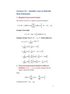
Lecture 12 -- Another way to find the Best Estimator
www.ams.sunysb.edu1 Lecture 12 -- Another way to find the Best Estimator 1. (Regular) Exponential Family The density function of a regular exponential family is:
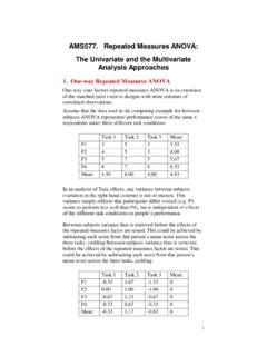
AMS577. Repeated Measures ANOVA: The …
www.ams.sunysb.edu1 AMS577. Repeated Measures ANOVA: The Univariate and the Multivariate Analysis Approaches 1. One-way Repeated Measures ANOVA One-way (one-factor) repeated-measures ANOVA is an extension
Repeated Measures ANOVA - Stony Brook
www.ams.sunysb.eduAs with any ANOVA, repeated measures ANOVA tests ... In the one-way analysis of variance without a repeated measure, we would have each subject receive

Examples: Joint Densities and Joint Mass Functions
www.ams.sunysb.eduAMS 311 Joe Mitchell Examples: Joint Densities and Joint Mass Functions Example 1: X and Y are jointly continuous with joint pdf f(x,y) = ˆ cx2 + xy 3 if 0 ≤ x ≤ 1, 0 ≤ y ≤ 2

Chapter 3: The basic concepts of probability - Stony Brook
www.ams.sunysb.eduChapter 3: The basic concepts of probability Experiment: a measurement process that produces quantifiable results (e.g. throwing two dice, dealing cards, at poker, measuring heights of people, recording proton-proton collisions)

Unit Root & Augmented Dickey-Fuller (ADF) Test
www.ams.sunysb.eduDickey-Fuller Tests • If a constant or trend belong in the equation we must also use D-F test stats that adjust for the impact on the distribution of the test statistic (* see problem set 3 where we included the drift/linear trend in the Augmented D-F test). • The D-F is generalized into the Augmented D-F test to accommodate the general

The Ordinary Least Squares (OLS) Estimator
www.ams.sunysb.eduGauss-Markov Theorem • Given OLS assumptions 1 through 6, the OLS estimator of β k is the minimum variance estimator from the set of all linear unbiased estimators of β

Solutions Manual for Statistical Inference, Second Edition
www.ams.sunysb.edusecond edition, problems were shuffled with no attention paid to numbering (hence no attention paid to minimize the new effort), but rather we tried to put the problems in logical order. A major change from the first edition is the use of the computer, both symbolically through Mathematicatm and numerically using R. Some solutions are given ...
Related documents
APPLIED ECONOMETRIC TIME SERIES (4th edition)
time-series.net1. Looking at the time path of a series is the single most important step in forecasting the series. Examining the series allows you to see if it has a clear trend and to get a reasonable idea if the trend is linear or nonlinear. Similarly, a series may or …

Lecture 13 Time Series: Stationarity, AR(p) & MA(q)
www.bauer.uh.eduRS –EC2 -Lecture 13 3 • We want to select an appropriate time series model to forecast yt. In this class, the choices are AR(p), MA(q) or ARMA(p, q). • Steps for forecasting: (1) Identify the appropriate model. That is, determine p, q. (2) Estimate the model. (3) Test the model.
Supply Chain Management: Forcasting techniques and ... - …
www2.unb.caForecast TechniquesII 2 Market research methods: Use market testing and surveys to predict particularly newly introduced products. 3 Quantitative forecasting: Time series model: uses historical data assuming the future will be like the past.

Seasonal Dummy Model - Social Science Computing …
www.ssc.wisc.edu• At any time period t, one of the seasonal dummies D ... • It is a complete forecasting model it t p t p t s i ... Fitted Values. Last 2 years. 12‐month forecast. Forecasting with Seasonal Dummy • To forecast in STATA with seasonal dummies, the ...
Slides on ARIMA models--Robert Nau - Duke University
people.duke.edu3 Construction of an ARIMA model 1. Stationarize the series, if necessary, by differencing (& perhaps also logging, deflating, etc.) 2. Study the pattern of autocorrelations and partial autocorrelations to determine if lags of the stationarized series and/or lags of the forecast errors should be included in the forecasting equation 3.

03 Time series with trend and seasonality components
web.vu.ltDetermining if a time series has a seasonal component Some examples of more pronounced seasonality: g = 1 Time z 0 40 80 120-4-2 0 2 4 0 5 10 15 20-0.5 0.0 0.5 1.0 Lag ACF Series z g = 0.83 Time z 0 40 80 120-4 4 0 5 10 15 20-0.5 1.0 Lag ACF Series z g = 0.5 Time z 0 40 80 120-3-1 1 2 3 0 5 10 15 20-0.5 0.0 0.5 1.0 Lag ACF Series z g = 0.25 ...

University of Pennsylvania
www.sas.upenn.edu5.3 Naive Accept-Reject Method94 10.1 Time Series of Daily NYSE Returns146 10.2 Correlogram of Daily NYSE Returns.147 10.3 Histogram and Statistics for Daily NYSE Returns.147 10.4 Time Series of Daily Squared NYSE Returns.148 10.5 Correlogram of Daily Squared NYSE Returns.148 10.6 True Exceedance Probabilities of Nominal 1% HS-VaRWhen Volatility

R and Data Mining: Examples and Case ... - University of Idaho
www.webpages.uidaho.eduMessages from the Author Case studies: The case studies are not included in this online version. They are reserved exclu-sively for a book version published by Elsevier in December 2012.