Transcription of VORTEX DYNAMICS 1. Introduction
1 VORTEX DYNAMICS1. IntroductionA VORTEX is commonly associated with the rotating motion of uid around acommon centerline. It is de ned by thevorticityin the uid, which measuresthe rate of local uid rotation. Typically, the uid circulates around the VORTEX ,the speed increases as the VORTEX is approached and the pressure decreases. Vor-tices arise in nature and technology in a large range of sizes as illustrated by theexamples given in Table 1. The next section presents some of the mathematicalbackground necessary to understand VORTEX formation and evolution.
2 Section 3describes sample ows, including important instabilities and reconnection pro-cesses. Section 4 presents some of the numerical methods used to simulate these uid vortices10 8cm (= 1 A)trailing VORTEX of Boeing 7271{2 mdust devils1{10 mtornadoes10{500 mhurricanes100{2000 kmJupiter's Red Spot25,000 kmspiral galaxiesthousands of light yearsTABLE 1: Sample vortices and typical BackgroundLetDbe a region in 3D space containing a uid, and letx=(x; y; z)Tbe apoint inD. The uid motion is described by its velocityu(x;t)=u(x;t)i+v(x;t)j+w(x;t)k, and depends on the uid density (x;t), temperatureT(x;t),gravitational eldgand other external forces possibly acting on it.}}}}
3 The uidvorticity is de ned by!!=r u. The vorticity measures the local uid rotationabout an axis, as can be seen by expanding the velocity nearx=x0,u(x)=u(x0)+D(x0)(x x0)+12!!(x0) (x x0)+O(jx x0j2) (1)whereD(x0)=12(ru+ruT);ru="uxuyuzvxvyv zwxwywz#:(2)The rst termu(x0) corresponds to translation: all uid particles move withconstant velocityu(x0). The second termD(x0)(x x0) corresponds to astrain eld in the three directions of the eigenvectors of the symmetric matrixD. If the eigenvalue corresponding to a given eigenvector is positive, the uid isstretched in that direction, if it is negative, the uid is compressed.
4 Note thatin incompressible owr u= 0, so the sum of the eigenvalues ofDequals (a)(b)Figure 1: Strain eld. (a) Two positive eigenvalues, sheet formation. (b) Onepositive eigenvalue, tube at least one eigenvalue is positive and one negative. If the third eigenvalueis positive, uid particles move towards sheets (Fig. 1a). If the third eigenvalueis negative, uid particles move towards tubes (Fig. 1b). The last term in Eq.(1),12!!(x0) (x x0), corresponds to a rotation: near a point with!!(x0)6=0,the uid rotates with angular velocityj!
5 !j=2 in a plane normal to the vorticityvector!!. Fluid for which!!=0is said to lineis an integral curve of the vorticity. For incompressible ow,r !!=r (r u) = 0 which implies that VORTEX lines cannot end in the interiorof the ow, but must either form a closed loop or start and end at a boundingsurface. In 2D ow,u=ui+vjand the vorticity is!!=!k, where!=vx uyis thescalar vorticity. Thus in 2D, the vorticity points in thez-direction andthe VORTEX lines are straight lines normal to thex-yplane. Avortex tubeis abundle of VORTEX lines.
6 Thestrengthof a VORTEX tube is de ned as thecirculationRCu dsabout a curveCenclosing the tube. By Stokes' Theorem,ZCu ds=ZZA!! ndS ;(3)and thus the circulation can also be interpreted as the ux of vorticity througha cross section of the tube. In inviscid incompressible ow of constant density,Helmholtz' Theoremstates that the tube strength is independent of the curveC, and is therefore a well-de ned quantity, andKelvin's Theoremstates that atube's strength remains constant in time. Avortex lamentis an idealizationin which a tube is represented by a single VORTEX line of nonzero evolution equation for the uid vorticity, as derived from the Navier-Stokes Equations, isd!
7 !dt=!! ru+ !!(4)where d=dt=@=@t+u ris the total time derivative. Equation (4) states thatthe vorticity is transported by the uid velocity ( rst term), stretched by the uid velocity gradient (second term), and di used by viscosity (last term).These equations are usually nondimensionalized and written in terms of theReynolds number, a dimensionless quantity inversely proportional to (a)(b)rdistancespeed |u|Figure 2: Flow induced by a point VORTEX . (a) Streamlines. (b) understand high Reynolds number ow it is of interest to study theinviscid Euler Equations.
8 The corresponding vorticity evolution equation in 2 Disd!!dt=0;(5)which states that 2D VORTEX laments in inviscid ow move with the uid veloc-ity. Furthermore, in incompressible ow the uid velocity is determined by thevorticity, up to an irrotational far- eld componentu1, through theBiot-Savartlaw,u(x)= 14 Z(x x0) !!(x0)jx x0j3dx0+u1:(6)In planar 2D ow, Eq (6) reduces tou(x)=K2d !;whereK2d(x)=12 yi+xjjxj2(7)and!(x) is the scalar vorticity. Equations (4,5) and (6,7) are the basis of thenumerical methods discussed typically de ned by a region in the uid of concentrated simple model is apoint vortexin 2D ow, which corresponds to a straightvortex lament of unit circulation.
9 The associated scalar vorticity is a deltafunction in the plane, and the induced velocity is obtained from the Biot-Savartlaw. For a point VORTEX at the origin this reduces to the radial velocity eldu(x)=K2d =K2d(x). Corresponding particle trajectories are shown in (a). The particle speedjuj=1=rincreases unboundedly as the VORTEX center isapproached, and vanishes asr!1(Fig. 2b). In general, the far eld velocityof a concentrated VORTEX behaves similarly to the one of a point VORTEX , withspeeds decaying as 1=r. Near the VORTEX center, the velocity typically increasesin magnitude and as a result, the uid pressure decreases (Bernoulli's Theorem).
10 A VORTEX of arbitrary shape can be approximated by a sum of point vortices (in2D) or VORTEX laments (in 3D), as is often done for simulation can be generated by a variety of mechanisms. For example, vortic-ity can be generated by density gradients, which in turn are induced by spatial3y Uuyd(a)(b)oFigure 3: Velocity and vorticity in boundary layer near a at variations. This mechanism explains the formation of warm-airvortices when a layer of hot air is trapped underneath cooler air. Vorticity isalso generated near solid walls in the form ofboundary layerscaused by viscos-ity.