Transcription of VORTEX DYNAMICS 1. Introduction
1 VORTEX DYNAMICS1. IntroductionA VORTEX is commonly associated with the rotating motion of uid around acommon centerline. It is de ned by thevorticityin the uid, which measuresthe rate of local uid rotation. Typically, the uid circulates around the VORTEX ,the speed increases as the VORTEX is approached and the pressure decreases. Vor-tices arise in nature and technology in a large range of sizes as illustrated by theexamples given in Table 1. The next section presents some of the mathematicalbackground necessary to understand VORTEX formation and evolution. Section 3describes sample ows, including important instabilities and reconnection pro-cesses. Section 4 presents some of the numerical methods used to simulate these uid vortices10 8cm (= 1 A)trailing VORTEX of Boeing 7271{2 mdust devils1{10 mtornadoes10{500 mhurricanes100{2000 kmJupiter's Red Spot25,000 kmspiral galaxiesthousands of light yearsTABLE 1: Sample vortices and typical BackgroundLetDbe a region in 3D space containing a uid, and letx=(x; y; z)Tbe apoint inD.}}}}
2 The uid motion is described by its velocityu(x;t)=u(x;t)i+v(x;t)j+w(x;t)k, and depends on the uid density (x;t), temperatureT(x;t),gravitational eldgand other external forces possibly acting on it. The uidvorticity is de ned by!!=r u. The vorticity measures the local uid rotationabout an axis, as can be seen by expanding the velocity nearx=x0,u(x)=u(x0)+D(x0)(x x0)+12!!(x0) (x x0)+O(jx x0j2) (1)whereD(x0)=12(ru+ruT);ru="uxuyuzvxvyv zwxwywz#:(2)The rst termu(x0) corresponds to translation: all uid particles move withconstant velocityu(x0). The second termD(x0)(x x0) corresponds to astrain eld in the three directions of the eigenvectors of the symmetric matrixD. If the eigenvalue corresponding to a given eigenvector is positive, the uid isstretched in that direction, if it is negative, the uid is compressed. Note thatin incompressible owr u= 0, so the sum of the eigenvalues ofDequals (a)(b)Figure 1: Strain eld.
3 (a) Two positive eigenvalues, sheet formation. (b) Onepositive eigenvalue, tube at least one eigenvalue is positive and one negative. If the third eigenvalueis positive, uid particles move towards sheets (Fig. 1a). If the third eigenvalueis negative, uid particles move towards tubes (Fig. 1b). The last term in Eq.(1),12!!(x0) (x x0), corresponds to a rotation: near a point with!!(x0)6=0,the uid rotates with angular velocityj!!j=2 in a plane normal to the vorticityvector!!. Fluid for which!!=0is said to lineis an integral curve of the vorticity. For incompressible ow,r !!=r (r u) = 0 which implies that VORTEX lines cannot end in the interiorof the ow, but must either form a closed loop or start and end at a boundingsurface. In 2D ow,u=ui+vjand the vorticity is!!=!k, where!=vx uyis thescalar vorticity. Thus in 2D, the vorticity points in thez-direction andthe VORTEX lines are straight lines normal to thex-yplane.
4 Avortex tubeis abundle of VORTEX lines. Thestrengthof a VORTEX tube is de ned as thecirculationRCu dsabout a curveCenclosing the tube. By Stokes' Theorem,ZCu ds=ZZA!! ndS ;(3)and thus the circulation can also be interpreted as the ux of vorticity througha cross section of the tube. In inviscid incompressible ow of constant density,Helmholtz' Theoremstates that the tube strength is independent of the curveC, and is therefore a well-de ned quantity, andKelvin's Theoremstates that atube's strength remains constant in time. Avortex lamentis an idealizationin which a tube is represented by a single VORTEX line of nonzero evolution equation for the uid vorticity, as derived from the Navier-Stokes Equations, isd!!dt=!! ru+ !!(4)where d=dt=@=@t+u ris the total time derivative. Equation (4) states thatthe vorticity is transported by the uid velocity ( rst term), stretched by the uid velocity gradient (second term), and di used by viscosity (last term).
5 These equations are usually nondimensionalized and written in terms of theReynolds number, a dimensionless quantity inversely proportional to (a)(b)rdistancespeed |u|Figure 2: Flow induced by a point VORTEX . (a) Streamlines. (b) understand high Reynolds number ow it is of interest to study theinviscid Euler Equations. The corresponding vorticity evolution equation in 2 Disd!!dt=0;(5)which states that 2D VORTEX laments in inviscid ow move with the uid veloc-ity. Furthermore, in incompressible ow the uid velocity is determined by thevorticity, up to an irrotational far- eld componentu1, through theBiot-Savartlaw,u(x)= 14 Z(x x0) !!(x0)jx x0j3dx0+u1:(6)In planar 2D ow, Eq (6) reduces tou(x)=K2d !;whereK2d(x)=12 yi+xjjxj2(7)and!(x) is the scalar vorticity. Equations (4,5) and (6,7) are the basis of thenumerical methods discussed typically de ned by a region in the uid of concentrated simple model is apoint vortexin 2D ow, which corresponds to a straightvortex lament of unit circulation.
6 The associated scalar vorticity is a deltafunction in the plane, and the induced velocity is obtained from the Biot-Savartlaw. For a point VORTEX at the origin this reduces to the radial velocity eldu(x)=K2d =K2d(x). Corresponding particle trajectories are shown in (a). The particle speedjuj=1=rincreases unboundedly as the VORTEX center isapproached, and vanishes asr!1(Fig. 2b). In general, the far eld velocityof a concentrated VORTEX behaves similarly to the one of a point VORTEX , withspeeds decaying as 1=r. Near the VORTEX center, the velocity typically increasesin magnitude and as a result, the uid pressure decreases (Bernoulli's Theorem).A VORTEX of arbitrary shape can be approximated by a sum of point vortices (in2D) or VORTEX laments (in 3D), as is often done for simulation can be generated by a variety of mechanisms. For example, vortic-ity can be generated by density gradients, which in turn are induced by spatial3y Uuyd(a)(b)oFigure 3: Velocity and vorticity in boundary layer near a at variations.
7 This mechanism explains the formation of warm-airvortices when a layer of hot air is trapped underneath cooler air. Vorticity isalso generated near solid walls in the form ofboundary layerscaused by viscos-ity. To illustrate, imagine horizontal ow with speedUomoving past a solid wallat rest (Fig. 3a). Since in viscous ow the uid sticks to the wall (the no-slipboundary condition), the uid velocity at the wall is zero. As a result, there isa thin layer near the wall in which the horizontal velocity varies greatly whilethe vertical velocity gradients are small, yielding large negative vorticity values!=vx uy(Fig. 3b). Similarity solutions to the approximatingPrandtl bound-ary layer equationsshow that the boundary layer thicknessdgrows proportionaltoptwheretmeasures the time from the beginning of the motion. Boundarylayers can separate from the wall at corners or regions of high curvature andmove into the uid interior, as illustrated in several of the following Sample VORTEX Shear layersA shear layer is a thin region of concentrated vorticity across which the tan-gential velocity component varies greatly.
8 An example is the constant vorticitylayer given by parallel 2D owu(x; y)=U(y),v(x; y) = 0, whereUis as shownin Fig. 4(a). In this case, the velocity is constant outside the layer and linearinside. The vorticity!= U0(y) is zero outside the layer and constant layers occur naturally in the ocean or atmosphere when regions of dis-tinct temperature or density meet. To illustrate this scenario, consider a tankcontaining two horizontal layers of uids of di erent densities, one on top of theother. If the tank is tilted, the heavier bottom uid moves downstream, andthe lighter one moves upstream, creating a shear shear layers are unstable to perturbations: they do not remain at butroll up into a sequence of vortices. This is theKelvin-Helmholtz instability, whichcan be deduced analytically using linear stability analysis. One shows that ina periodically perturbed at shear layer, the amplitude of a perturbation withwavenumberkwill initially grow exponentially in time asewt, wherew=w(k)is thedispersion relation, leading to instability.
9 Thewavenumber oflargestgrowth depends on the layer thickness. This is illustrated in Fig. 4(b), (a) (b)wFigure 4: Shear layer. (a) Velocity pro le. (b) Dispersion (a)wk(b)Figure 5: VORTEX sheet. (a) Velocity pro le. (b) Dispersion 6: Computation of VORTEX sheet 7: Sketch. Shear layer separation and roll-up into trailing vortices behindan (k) for a constant vorticity layer of thickness 2d. The wavenumber ofmaximal growth is proportional to 1= VORTEX sheet is a model for a shear layer. The layer is approximated by asurface of zero thickness across which the tangential velocity is discontinuous,as illustrated in Fig. 5(a). In this case the dispersion relation reduces tow(k)= k:That is, for eachwavenumberkthere is a growing and a decaying mode,and the growing mode grows faster the higher thewavenumber is, as shownin Fig. 5(b). The VORTEX sheet arises from a constant vorticity shear layer asthe thicknessd!
10 0 and the vorticity!!1in such a way that the product!dremains constant. Figure 6 shows the roll-up of a periodically perturbedvortex sheet due to the Kelvin-Helmholtz instability, computed using one of themethods described Aircraft trailing vorticesOne can often observe trailing vortices that shed from the wings of a yingaircraft (also called contrails). These vortices are formed because the wingdevelops lift. The pressure on the top of the wing is lower than on bottom,causing air to move around the edge of the wing from the bottom surface tothe top. The boundary layer on the wing separates as a shear layer that rollsup into a VORTEX attached to the tip of the wing (Fig. 7). Since the velocityinside the VORTEX is high, the pressure is correspondingly low and causes watervapor in the air to condense, forming water droplets that visualize the VORTEX strength increases with increasing lift, and is particularly strong inhigh-lift conditions such as take-o and landing.