Transcription of Wasserstein Generative Adversarial Networks
1 Wasserstein Generative Adversarial NetworksMartin Arjovsky1 Soumith Chintala2L eon Bottou1 2 AbstractWe introduce a new algorithm named WGAN,an alternative to traditional GAN training. Inthis new model, we show that we can improvethe stability of learning, get rid of problems likemode collapse, and provide meaningful learningcurves useful for debugging and hyperparametersearches. Furthermore, we show that the cor-responding optimization problem is sound, andprovide extensive theoretical work highlightingthe deep connections to different distances be-tween IntroductionThe problem this paper is concerned with is that of unsu-pervised learning. Mainly, what does it mean to learn aprobability distribution? The classical answer to this is tolearn a probability density. This is often done by defininga parametric family of densities(P ) Rdand finding theone that maximized the likelihood on our data: if we havereal data examples{x(i)}mi=1, we would solve the problemmax Rd1mm i=1logP (x(i))If the real data distributionPradmits a density andP is thedistribution of the parametrized densityP , then, asymp-totically, this amounts to minimizing the Kullback-LeiblerdivergenceKL(Pr P ).
2 For this to make sense, we need the model densityP toexist. This is not the case in the rather common situationwhere we are dealing with distributions supported by lowdimensional manifolds. It is then unlikely that the modelmanifold and the true distribution s support have a non-negligible intersection (see (Arjovsky & Bottou, 2017)),and this means that the KL distance is not defined (or sim-ply infinite).1 Courant Institute of Mathematical Sciences, NY2 FacebookAI Research, NY. Correspondence to: Martin of the34thInternational Conference on MachineLearning, Sydney, Australia, PMLR 70, 2017. Copyright 2017by the author(s).The typical remedy is to add a noise term to the model dis-tribution. This is why virtually all Generative models de-scribed in the classical machine learning literature includea noise component. In the simplest case, one assumes aGaussian noise with relatively high bandwidth in order tocover all the examples.
3 It is well known, for instance, thatin the case of image generation models, this noise degradesthe quality of the samples and makes them blurry. For ex-ample, we can see in the recent paper (Wu et al., 2016)that the optimal standard deviation of the noise added tothe model when maximizing likelihood is around toeach pixel in a generated image, when the pixels were al-ready normalized to be in the range[0,1]. This is a veryhigh amount of noise, so much that when papers report thesamples of their models, they don t add the noise term onwhich they report likelihood numbers. In other words, theadded noise term is clearly incorrect for the problem, but isneeded to make the maximum likelihood approach than estimating the density ofPrwhich may not ex-ist, we can define a random variableZwith a fixed dis-tributionp(z)and pass it through a parametric functiong :Z X(typically a neural network of some kind)that directly generates samples following a certain distribu-tionP.
4 By varying , we can change this distribution andmake it close to the real data distributionPr. This is use-ful in two ways. First of all, unlike densities, this approachcan represent distributions confined to a low dimensionalmanifold. Second, the ability to easily generate samples isoften more useful than knowing the numerical value of thedensity (for example in image superresolution or semanticsegmentation when considering the conditional distributionof the output image given the input image). In general, itis computationally difficult to generate samples given anarbitrary high dimensional density (Neal, 2001).Variational Auto-Encoders (VAEs) (Kingma & Welling,2013) and Generative Adversarial Networks (GANs)(Goodfellow et al., 2014) are well known examples of thisapproach. Because VAEs focus on the approximate likeli-hood of the examples, they share the limitation of the stan-dard models and need to fiddle with additional noise offer much more flexibility in the definition of theobjective function, including Jensen-Shannon (Goodfellowet al.)
5 , 2014), and allf-divergences (Nowozin et al., 2016)as well as some exotic combinations (Huszar, 2015). OnWasserstein Generative Adversarial Networksthe other hand, training GANs is well known for being del-icate and unstable, for reasons theoretically investigated in(Arjovsky & Bottou, 2017).In this paper, we direct our attention on the various ways tomeasure how close the model distribution and the real dis-tribution are, or equivalently, on the various ways to definea distance or divergence (P ,Pr). The most fundamen-tal difference between such distances is their impact on theconvergence of sequences of probability distributions. Asequence of distributions(Pt)t Nconverges if and only ifthere is a distributionP such that (Pt,P )tends to zero,something that depends on how exactly the distance isdefined. Informally, a distance induces a weaker topol-ogy when it makes it easier for a sequence of distributionto 2 clarifies how popular probabilitydistances differ in that order to optimize the parameter , it is of course desir-able to define our model distributionP in a manner thatmakes the mapping 7 P continuous.
6 Continuity meansthat when a sequence of parameters tconverges to , thedistributionsP talso converge toP . However, it is essen-tial to remember that the notion of the convergence of thedistributionsP tdepends on the way we compute the dis-tance between distributions. The weaker this distance, theeasier it is to define a continuous mapping from -space toP -space, since it s easier for the distributions to main reason we care about the mapping 7 P to becontinuous is as follows. If is our notion of distance be-tween two distributions, we would like to have a loss func-tion 7 (P ,Pr)that is continuous, and this is equivalentto having the mapping 7 P be continuous when usingthe distance between distributions .The contributions of this paper are: In Section 2, we provide a comprehensive theoreticalanalysis of how the Earth Mover (EM) distance be-haves in comparison to popular probability distancesand divergences used in the context of learning distri-butions.
7 In Section 3, we define a form of GAN calledWasserstein-GAN that minimizes a reasonable and ef-ficient approximation of the EM distance, and we the-oretically show that the corresponding optimizationproblem is sound. In Section 4, we empirically show that WGANs curethe main training problems of GANs. In particular,training WGANs does not require maintaining a care-ful balance in training of the discriminator and the1 More exactly, the topology induced by is weaker than thatinduced by when the set of convergent sequences under is asuperset of that under .generator, does not require a careful design of the net-work architecture either, and also reduces the modedropping that is typical in GANs. One of the mostcompelling practical benefits of WGANs is the abilityto continuously estimate the EM distance by trainingthe discriminator to optimality. Because they correlatewell with the observed sample quality, plotting theselearning curves is very useful for debugging and hy-perparameter Different DistancesWe now introduce our notation.
8 LetXbe a compact metricset, say the space of images[0,1]d, and let denote theset of all the Borel subsets ofX. Let Prob(X)denote thespace of probability measures defined onX. We can nowdefine elementary distances and divergences between twodistributionsPr,Pg Prob(X): TheTotal Variation(TV) distance (Pr,Pg) = supA |Pr(A) Pg(A)|. TheKullback-Leibler(KL) divergenceKL(Pr Pg) = log(Pr(x)Pg(x))Pr(x)d (x),where bothPrandPgare assumed to admit densitieswith respect to a same measure defined divergence is famously assymetric and possiblyinfinite when there are points such thatPg(x) = 0andPr(x)>0. TheJensen-Shannon(JS) divergenceJS(Pr,Pg) =KL(Pr Pm) +KL(Pg Pm),wherePmis the mixture(Pr+Pg)/2. This diver-gence is symmetrical and always defined because wecan choose =Pm. TheEarth-Mover(EM) distance or Wasserstein -1W(Pr,Pg) =inf (Pr,Pg)E(x,y) [ x y ],(1)where (Pr,Pg)is the set of all joint distributions (x,y)whose marginals are , (x,y)indicates how much mass mustbe transported fromxtoyin order to transform thedistributionsPrinto the distributionPg.
9 The EM dis-tance then is the cost of the optimal transport that a probability distributionPr Prob(X)admitsa densityPr(x)with respect to , that is, A ,Pr(A) = APr(x)d (x), if and only it is absolutely continuous with re-spect to , that is, A , (A) = 0 Pr(A) = Generative Adversarial NetworksFigure 1: These plots show (P ,P0)as a function of when is the EM distance (left plot) or the JS divergence (right plot). The EMplot is continuous and provides a usable gradient everywhere. The JS plot is not continuous and does not provide a usable following example illustrates how apparently simplesequences of probability distributions converge under theEM distance but do not converge under the other distancesand divergences defined 1(Learning parallel lines).LetZ U[0,1]theuniform distribution on the unit interval. LetP0be the dis-tribution of(0,Z) R2(a 0 on the x-axis and the randomvariableZon the y-axis), uniform on a straight vertical linepassing through the origin.
10 Now letg (z) = ( ,z)with a single real parameter. It is easy to see that in this case, W(P0,P ) =| |, JS(P0,P ) ={log 2if 6= 0,0if = 0, KL(P P0) =KL(P0 P ) ={+ if 6= 0,0if = 0, and (P0,P ) ={1if 6= 0,0if = t 0, the sequence(P t)t Nconverges toP0un-der the EM distance, but does not converge at all undereither the JS, KL, reverse KL, or TV divergences. Figure 1illustrates this for the case of the EM and JS 1 gives a case where we can learn a probabilitydistribution over a low dimensional manifold by doing gra-dient descent on the EM distance. This cannot be done withthe other distances and divergences because the resultingloss function is not even continuous. Although this simpleexample features distributions with disjoint supports, thesame conclusion holds when the supports have a non emptyintersection contained in a set of measure zero. This hap-pens to be the case when two low dimensional manifoldsintersect in general position (Arjovsky & Bottou, 2017).}}}