Convolution solutions (Sect. 6.6). Convolution of two ...

Thomas Calculus; 12th Edition: The Power Rule

Thomas Calculus; 12th Edition: The Power Rule Cli ord E. Weil September 15, 2010 The following paragraph appears at the bottom of page 116 of Thomas Calculus, 12th Edition. The Power Rule is actually valid for all real numbers n.

  Power, Edition, Thomas, Calculus, The power, 12th, Thomas calculus 12th edition, 12th edition, Thomas calculus

Convolution solutions (Sect. 6.6). - users.math.msu.edu

Convolution solutions (Sect. 6.6). I Convolution of two functions. I Properties of convolutions. I Laplace Transform of a convolution. I Impulse response solution. I Solution decomposition theorem.

Special Second Order Equations (Sect. 2.2). Special Second ...

Special Second Order Equations (Sect. 2.2). I Special Second order nonlinear equations. I Function y missing. (Simpler) I Variable t missing. (Harder) I Reduction order method. Special Second order nonlinear equations Definition Given a functions f : R3 → R, a second order differential equation in the unknown function y : R → R is given by

  Second, Special, Order, Equations, Sect, Second order, Special second order equations, Special second order

second order equations{Undetermined Coe - cients

September 29, 2013 9-1 9. Particular Solutions of Non-homogeneous second order equations{Undetermined Coe -cients We have seen that in order to nd the general solution to

  Second, Order, Equations, Undetermined, Second order equations undetermined

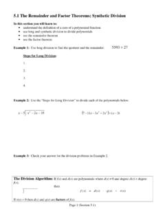
5.1 The Remainder and Factor Theorems.doc; Synthetic Division

Page 2 (Section 5.1) Example 4: Perform the operation below. Write the remainder as a rational expression (remainder/divisor). 2 1 2 8 2 3 5 4 3 2 + − + + x x x x x Synthetic Division – Generally used for “short” division of polynomials when the divisor is in the form x – c. (Refer to page 506 in your textbook for more examples.)

  Factors, Theorem, Remainder, The remainder and factor theorems

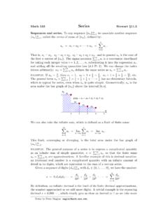
Math 133 Series Sequences and series. fa g

Geometric sequences and series. A general geometric sequence starts with an initial value a 1 = c, and subsequent terms are multiplied by the ratio r, so that a n = ra n 1; explicitly, a n = crn 1. The same trick as above gives a formula for the corresponding geometric series. We have s …

  Series, Sequence, Geometric, Geometric sequences and series, Geometric series, Series sequences and series

The Laplace Transform (Sect. 6.1). - users.math.msu.edu

The Laplace Transform (Sect. 6.1). I The definition of the Laplace Transform. I Review: Improper integrals. I Examples of Laplace Transforms. I A table of Laplace Transforms. I Properties of the Laplace Transform. I Laplace Transform and differential equations.

  Transform, Laplace transforms, Laplace, The laplace transform

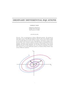
ORDINARY DIFFERENTIAL EQUATIONS

The equations in examples (c) and (d) are called partial di erential equations (PDE), since the unknown function depends on two or more independent variables, t, x, y, and zin these examples, and their partial derivatives appear in the equations.

  Differential, Equations, Variable, Ordinary, Ordinary differential equations

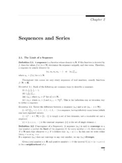
Sequences and Series - Michigan State University

2 2. Sequences and Series A topological way to say lima n = ais the following: Given any -neighborhood V (a) of a, there exists a place in the sequence after which all of the terms are in V (a): Easy Fact: lim(c) = cfor all constant sequences (c): Quanti ers. The de nition of lima n = aquanti es the closeness of a n to aby an arbi-

  Series, Sequence, Sequences and series

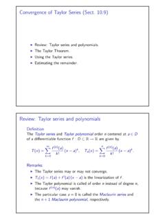
Convergence of Taylor Series (Sect. 10.9) Review: Taylor ...

Convergence of Taylor Series (Sect. 10.9) I Review: Taylor series and polynomials. I The Taylor Theorem. I Using the Taylor series. I Estimating the remainder. The Taylor Theorem Remark: The Taylor polynomial and Taylor series are obtained from a generalization of the Mean Value Theorem: If f : [a,b] → R is differentiable, then there exits c ∈ (a,b) such that

  Review, Convergence

Laplace Transform solved problems - cuni.cz

Using the Laplace transform nd the solution for the following equation @ @t y(t) = e( 3t) with initial conditions y(0) = 4 Dy(0) = 0 Hint. no hint Solution. We denote Y(s) = L(y)(t) the Laplace transform Y(s) of y(t). We perform the Laplace transform for both sides of the given equation. For particular functions we use tables of the Laplace ...

  Solutions, Transform, Laplace transforms, Laplace

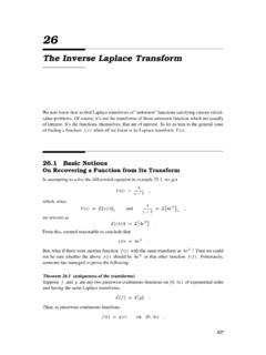
The Inverse Laplace Transform

532 The Inverse Laplace Transform! Example 26.5: In exercise25.1e on page 523, you found thatthe Laplacetransformof the solution to y′′ + 4y = 20e4t with y(0) = 3 and y′(0) = 12 is Y(s) = 3s2 −28 (s −4). s2 +4 The partial fraction expansion of this is Y(s) = 3s2 −28 (s − 4) s2 +4 A s − + Bs +C s2 +4 for some constants A, B and C .

  Solutions, Transform, Laplace transforms, Laplace

ELEMENTARY DIFFERENTIAL EQUATIONS

Chapter 8 Laplace Transforms 8.1 Introduction to the Laplace Transform 394 8.2 The Inverse Laplace Transform 406 8.3 Solution ofInitial Value Problems 414 8.4 The Unit Step Function 421 8.5 Constant Coefficient Equationswith Piecewise Continuous Forcing Functions 431 8.6 Convolution 441 8.7 Constant Cofficient Equationswith Impulses 453

  Solutions, Differential, Equations, Elementary, Transform, Elementary differential equations, Laplace transforms, Laplace

1 Z-Transforms, Their Inverses Transfer or System Functions

If you don’t know what a Laplace transform is, you aren’t missing anything that will help you. The above three properties still hold, but computing X(z) now requires use of: ... Solution: Take the z-transforms of the difference equation and of the input. This yields Y(z) −2z−1Y(z) = z−1X(z)−z−2X(z); X(z) = z z −3

  Solutions, Transform, Laplace transforms, Laplace

Chapter 13: The Laplace Transform in Circuit Analysis

solution satisfied the given initial conditions and final behavior. ... Transfer Function: the s-domain ratio of the Laplace transform of the output (response) to the Laplace transform of the input (source) ℒ ℒ Example. Finding the transfer function of an RLC circuit If the voltage is the desired output: ...

  Solutions, Transform, Laplace transforms, Laplace

Solving Differential Equations Using Simulink

Jul 01, 2019 · related to the Laplace transform L Z t 0 f(t)dt = 1 s F(s), where F(s) is the Laplace transform of f(t). integrate dx dt, producing x(t). introduction to simulink 3 ... The solution shown in Figure 1.13 had a setting of 1 and that in Figure 1.16 …

  Solutions, Transform, Laplace transforms, Laplace

TABLE OF INVERSE LAPLACE TRANSFORMS

first- and second-order equations, followed by Chapter 5 (the Laplace transform), Chapter 6 (systems), Chapter 8 (nonlinear equations), and part of Chapter 9 (partial differential equations). I generally spend a couple of days giving a rough overview of the omitted chapters: series solutions (Chapter 4) and difference equations (Chapter 7).

  Transform, Laplace transforms, Laplace

Solution of ODEs using Laplace Transforms - Queen's U

Solution of ODEs We can continue taking Laplace transforms and generate a catalogue of Laplace domain functions. The final aim is the solution of ordinary differential equations. Example Using Laplace Transform, solve Result

  Solutions, Transform, Laplace transforms, Laplace

Lecture #7 Lagrange's Equations - MIT OpenCourseWare

Laplace, Legendre (Newton 1643-1727) • Contributions o Calculus of variations ... Example: Work in polar coordinates, then transform to rectangular coordinates, e.g. sin cos ... Existence of constraints complicates the solution of the problem.

  Solutions, Mit opencourseware, Opencourseware, Transform, Laplace

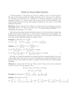
Section 7.4: Inverse Laplace Transform - University of Florida

nding inverse Laplace transforms is a critical step in solving initial value problems. To determine the inverse Laplace transform of a function, we try to match it with the form of an entry in the right-hand column of a Laplace table. Example 1. Determine L 1fFgfor (a) F(s) = 2 s3, (b) F(s) = 3 s 2+ 9, (c) F(s) = s 1 s 2s+ 5. Solution. (a) L 21 ...

  Solutions, Transform, Laplace transforms, Laplace