Lecture 9: Intercept Point, Gain Compression and Blocking
Finally, equating the cubic terms we have 0 = a1b3 +a22b1b2 +a3b 3 1 b3 = 2a2 2 a5 1 − a3 a4 1 It’s interesting to note that if one power series does not have cubic, a3 ≡ 0, the inverse series has cubic due to the first term above. A. M. Niknejad University of California, Berkeley EECS 142 Lecture 9 …
Download Lecture 9: Intercept Point, Gain Compression and Blocking

Information
Domain:
Source:
Link to this page:
Documents from same domain
EECS 242
rfic.eecs.berkeley.eduEECS 242 Scattering Parameters Prof. Niknejad University of California, Berkeley University of California, Berkeley EECS 242 – p. 1/43
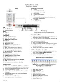
myDAQ How-to Guide
rfic.eecs.berkeley.eduLeland Au 1 myDAQ How-to Guide Leland Au, UC Berkeley Intro USB: 1. Type B USB port 2. Blue LED Indicator Audio: 3.
Class E/F Amplifiers - University of California, Berkeley
rfic.eecs.berkeley.eduClass A/B/C Properties Keep voltage waveform sinusoidal amplitude is limited to V dd /2 Only way to improve efficiency is to control current Require very large “on” current to deliver power EECS 242 Prof. Ali M. Niknejad (C) 2009

Power Amplifiers for Communications
rfic.eecs.berkeley.eduPeak E ciency Power Added E ciency (PAE) is a popular metric. P out is the output power, P in is the input power, and P dc is the DC power consumption of the PA For high power gain systems (G p), the e ciency approaches the drain drain e ciency ( d), or for a BJT, the \collector" e ciency, or simply the e ciency of the last stage

EECS 242: Mixer Noise and Design
rfic.eecs.berkeley.eduThe mixer voltage gain is the ratio of the output voltage signal at the IF frequency to the RF input voltage signal. If the LO is at either peak, one
Lecture 12: Noise in Communication Systems
rfic.eecs.berkeley.eduThe noise of the first stage is the most important. Thus, every communication system employs a low noise amplifier (LNA) at the front to relax the noise requirements A typical LNA might have a G = 20dB of gain and a noise figure NF < 1.5dB. …

Phase Locked Loops (PLL) and Frequency Synthesis
rfic.eecs.berkeley.edudivider between N and N + 1 using a sigma-delta modulator. In practice, the programmable divider is made of up ... is an important fact to consider when designing a PLL. Niknejad PLLs and Frequency Synthesis. Divider Linear Model From …

Lecture 15: Introduction to Mixers
rfic.eecs.berkeley.eduImage Reject Filter In our example, RF = 1000MHz, and IF = 1MHz.The Imagine is on 2IF = 2MHz away. Let’s design a filter with f0 = 1000MHz and f1 = 1001MHz. A fifth-order Chebyshev filter with 0.2dB ripple is down about 80dB at the IF frequency. But the Q for such a filter is Q = 103MHz 1MHz = 103 Such a filter requires components with Q > 103! A. M. Niknejad …
Nonlinear System Theory
rfic.eecs.berkeley.eduphase-plane analysis describes nonlinear phenomena such as limit cycles and multiple equilibria of second-order systems in an efficient manner. The theory of differential equations has led to a highly developed stability theory for some classes of nonlinear systems. (Though, of course, an engineer cannot live by stability alone.) Functional
Crystal Oscillators (XTAL) - University of California ...
rfic.eecs.berkeley.eduSeries and Parallel Mode C 0 L 1 C 1 R 1 C 0 L 1 R 1 low resistance high resistance Due to the external physical capacitor, there are two resonant modes between a series branch and the capacitor. In the series mode ωs, the LCR is a low impedance (“short”). But beyond this frequency, the LCR is an equivalent inductor that resonates
Related documents

Cubic equations - mathcentre.ac.uk
www.mathcentre.ac.ukSolving cubic equations Now let us move on to the solution of cubic equations. Like a quadratic, a cubic should always be re-arranged into its standard form, in this case ax3 +bx2 +cx+d = 0 The equation x2 +4x− 1 = 6 x is a cubic, though it is not written in the standard form. We need to multiply through by x,

Graphing Polynomial Functions
static.bigideasmath.comSection 4.1 Graphing Polynomial Functions 161 Solving a Real-Life Problem The estimated number V (in thousands) of electric vehicles in use in the United States can be modeled by the polynomial function V(t) = 0.151280t3 − 3.28234t2 + 23.7565t − 2.041 where t represents the year, with t = 1 corresponding to 2001. a. Use a graphing calculator to graph the function for …
Instructor’s Solution Manual for Fundamentals of Physics ...
bayanbox.ir2. The customer expects 20×7056 in3 and receives 20×5826 in3, the difference being 24600 cubic inches, or 3 24600 in3 2.54 cm 1 inch 1 L 1000 cm3 = 403 L where Appendix D has been used (see also Sample Problem 1-2). 3. Using the given conversion factors, we find (a) the distance din rods to be d= 4.0furlongs = (4.0furlongs)(201.168m/furlong ...

Asymptotic Analysis and Singular Perturbation Theory
www.math.ucdavis.eduSolving the leading-order perturbation equation, we obtain the three roots x 0 = 0; 1: Solving the rst-order perturbation equation, we nd that x 1 = 1 ... We only obtain one solution because the cubic equation (1.4) degenerates to a linear equation at "= 0. We missed the other two solutions because they approach in nity

Chapter 10 – Isoparametric Elements - Memphis
www.ce.memphis.eduthe twelve-noded cubic quadrilateral (Q12) element • To compare the performance of the CST, Q4, Q6, Q8, and Q9 elements to beam elements CIVL 7/8117 Chapter 10 – Isoparametric Elements 1/108. Isoparametric Elements Introduction ... Solving for the a's in terms of x1and x2, ...

Solving Cubic Polynomials - SHSU
www.shsu.eduSolving Cubic Polynomials 1.1 The general solution to the quadratic equation There are four steps to nding the zeroes of a quadratic polynomial. 1.First divide by the leading term, making the polynomial monic. 2.Then, given x2 + a 1x+ a 0, substitute x= y a 1 2 to obtain an equation without the linear term. (This is the \depressed" equation.)

IEEE TRANSACTIONS Cubic Convolution Interpolation for ...
ncorr.comas the method of cubic splines. The spline interpolation kernel is not zero for nonzero integers. As a result, the ck’s must be determined by solving a matrix problem. In addition to being 0 or 1 at the interpolation nodes, the in- terpolation kernel must …

Cubic and Quartic Functions
www.cambridge.edu.auTo find equations for given cubic graphs. To apply cubic and quartic functions to solving problems. To use finite difference tables to find rules of sequences generated by polynomial functions. In Chapter 4 we looked at second degree polynomials or quadratics. A third degree polynomial is called a cubic and is a function, f, with rule