
MATH 304 Linear Algebra
MATH 304 Linear Algebra Lecture 14: Basis and coordinates. Change of basis. Linear transformations. Basis and dimension Definition. Let V be a vector space. A linearly independent spanning set for V is called a basis. Theorem Any vector space V has a basis. If V ... 0 1 1 . The ...
Download MATH 304 Linear Algebra

Information
Domain:
Source:
Link to this page:
Documents from same domain

Thales of Miletus1 - Texas A&M University
www.math.tamu.eduThales 2 • Thales of Miletus was the first known Greek philosopher, scientist and mathematician. Some consider him the teacher of Pythagoras, though it may be only be that he advised Pythagoras to travel to

Matrices and Linear Algebra - Texas A&M University
www.math.tamu.eduChapter 2 Matrices and Linear Algebra 2.1 Basics Definition 2.1.1. A matrix is an m×n array of scalars from a given field F. The individual values in the matrix are called entries.
Solving ODE in MATLAB - Texas A&M University
www.math.tamu.edu1.1 First Order Equations Though MATLAB is primarily a numerics package, it can certainly solve straightforward differential equations symbolically.1 Suppose, for example, that we want to solve the first

LYX 1.4.1 Basics - Texas A&M University
www.math.tamu.eduM442 LyX 1.4.1 P. Howard 3 LYX Basics 3.1 Creating a Simple Document LYX should splash up a simple logo over a gray screen. If the screen isn’t maximized, you

Partial Differential Equations in MATLAB 7 - Texas …
www.math.tamu.edufunction [pl,ql,pr,qr] = bc1(xl,ul,xr,ur,t) %BC1: MATLAB function M-file that specifies boundary conditions %for a PDE in time and one space dimension.

7KH %HJLQQLQJ - Texas A&M University
www.math.tamu.eduThe History of Infinity Definition 1. A point is that which has not part. Definition 4. A straight line is a line which lies evenly with the points on itself.
SYSTEMS OF LINEAR EQUATIONS AND 2 MATRICES
www.math.tamu.edu68 2 SYSTEMS OF LINEAR EQUATIONS AND MATRICES Systems of Equations Recall that in Section 1.4 we had to solve two simultaneous linear equations in order to find the break-even pointand the equilibrium point.

Taylor Series in MATLAB - Texas A&M University
www.math.tamu.eduTaylor Series in MATLAB First, let’s review our two main statements on Taylor polynomials with remainder. Theorem 1. (Taylor polynomial with integral remainder) Suppose a function f(x) and its

MATH 151 FALL SEMESTER 2011 COMMON …
www.math.tamu.edu4. Find the scalar projection (component) and vector projection of v 5i 12j onto w 4i 3j. a. scalar projection 16 13 vector projection 64 169 i 48 169 j b. scalar projection 16 13 vector projection 80
MATH 151, FALL 2009 COMMON EXAM II - …
www.math.tamu.eduPART II WORK OUT Directions: Present your solutions in the space provided. Show all your work neatly and concisely and Box your final answer. You will be graded not merely on the final answer, but also on the quality and correctness of the work
Related documents

Exercises in Digital Signal Processing 1 The Discrete ...
eeweb.poly.eduExercises in Digital Signal Processing Ivan W. Selesnick January 27, 2015 Contents 1 The Discrete Fourier Transform1 2 The Fast Fourier Transform16 3 Filters18 ... (1, 0, -1, 0). The length of the sequence is N= 4K. Simplify your answer. 4. 1.30The following MATLAB commands de ne …

1 True/False - University of Colorado Boulder
euclid.colorado.edu1 True/False True or false:Answers in blue. Justi cation is given unless the result is a direct statement of a theorem from the book/homework. 1.If a system of equations has fewer equations than unknowns, then it …

Chapter 1 Solutions to Review Problems
faculty.atu.edu2 CHAPTER 1. SOLUTIONS TO REVIEW PROBLEMS Exercise 44 Solve each of the following systems using the method of elimination: (a) ˆ 4x 1 −3x 2 = 0 2x 1 +3x 2 = 18 (b) ˆ 4x
34 Cubic Spline Approximation Problem:Given n x y i 0,1 ...
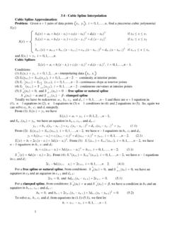
macs.citadel.eduExample Let f x cos x2 , x0 0, x1 0.6, and x2 0.9. Find a free cubic spline and a clamped cubic spline. 1. Free cubic spline: (I) Set up the 3 3matrixA and the 3 1 vector v: h0 0.6, h1 0.3 A 100 0.6 2 0.6 0.3 0…

SOLUTION FOR HOMEWORK 5, STAT 4351
utdallas.eduRemark: It can be a good habit to check you answer via verifying that the marginal density is integrated to 1. Let us do this: Z ∞ fX(x)dx = Z 1 0 (1/4)(4x+2)dx

Examples: Joint Densities and Joint Mass Functions
www.ams.sunysb.eduAMS 311 Joe Mitchell Examples: Joint Densities and Joint Mass Functions Example 1: X and Y are jointly continuous with joint pdf f(x,y) = ˆ cx2 + xy 3 if 0 ≤ x ≤ 1, 0 ≤ y ≤ 2

JP 1-0, Joint Personnel Support - Joint Chiefs of Staff
www.jcs.milJoint publication (JP) 1-0, Joint Personnel Support, is the foundational doctrine in the joint personnel series and represents our commitment to effective, integrated personnel support as a linchpin component of operational readiness.
Solutions to Exam 1 - Johns Hopkins University
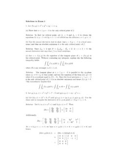
www.math.jhu.eduequations 2x+y ¡1 = 0;2y +x+1 = 0 which has the solution x = 1;y = ¡1. (b) Use the second derivative test to show that x = 1 ;y = ¡ 1 is a local mini- mum (and thus an absolute minimum it is the only critical point) of f .

Section 3.1: 12, 13, 20, 22 - Kent State University
www.math.kent.edu1 0, c 2 1/2. Therefore the solution to the IVP is y t 1/2sin2t. As t increases, the solution behave like steady oscillation. 18. y" 4y 5y 0,y 0 1,y 0 0. Solution The characteristic equation is r2 4r 5 0, r 1,2 4 16 20 2 2 i. Thus the general solution is given by y t c 1e 2t cos t c 2e 2t sin t. Take derivative
6. L’Hˆopital’s Rule - » Department of Mathematics
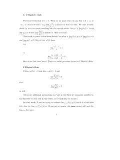
www.math.toronto.eduSometimes, L’Hˆopital’s Rule needs to be applied more than once; e.g., checking that we still have a 0/0 form each time before we apply the derivative to both numerator and
Related search queries
Exercises in Digital Signal Processing 1, Exercises in Digital Signal Processing, Chapter 1 Solutions to Review Problems, CHAPTER 1. SOLUTIONS TO REVIEW PROBLEMS, Cubic Spline Approximation Problem, SOLUTION FOR HOMEWORK 5, STAT 4351, Examples: Joint Densities and Joint Mass Functions, 1-0, Joint Personnel Support, Solutions to Exam 1, 6. L’Hˆopital’s Rule, L’Hˆopital’s Rule