
Multiple Life Models
xy is the probability that at least one of lives (x) and (y) will be alive after tyears. In contrast: t xy q is the probability that at least one of lives (x) and (y) will be dead within tyears. t q xy is the probability that both lives (x) and (y) will be dead within t years. Lecture: Weeks 9-10 (STT 456)Multiple Life ModelsSpring 2015 ...
Download Multiple Life Models

Information
Domain:
Source:
Link to this page:
Documents from same domain
Thomas Calculus; 12th Edition: The Power Rule
users.math.msu.eduThomas Calculus; 12th Edition: The Power Rule Cli ord E. Weil September 15, 2010 The following paragraph appears at the bottom of page 116 of Thomas Calculus, 12th Edition. The Power Rule is actually valid for all real numbers n.
Convolution solutions (Sect. 6.6). - users.math.msu.edu
users.math.msu.eduConvolution solutions (Sect. 6.6). I Convolution of two functions. I Properties of convolutions. I Laplace Transform of a convolution. I Impulse response solution. I Solution decomposition theorem.
Special Second Order Equations (Sect. 2.2). Special Second ...
users.math.msu.eduSpecial Second Order Equations (Sect. 2.2). I Special Second order nonlinear equations. I Function y missing. (Simpler) I Variable t missing. (Harder) I Reduction order method. Special Second order nonlinear equations Definition Given a functions f : R3 → R, a second order differential equation in the unknown function y : R → R is given by
second order equations{Undetermined Coe - cients
users.math.msu.eduSeptember 29, 2013 9-1 9. Particular Solutions of Non-homogeneous second order equations{Undetermined Coe -cients We have seen that in order to nd the general solution to
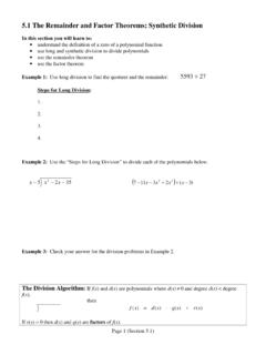
5.1 The Remainder and Factor Theorems.doc; Synthetic Division
users.math.msu.eduPage 2 (Section 5.1) Example 4: Perform the operation below. Write the remainder as a rational expression (remainder/divisor). 2 1 2 8 2 3 5 4 3 2 + − + + x x x x x Synthetic Division – Generally used for “short” division of polynomials when the divisor is in the form x – c. (Refer to page 506 in your textbook for more examples.)
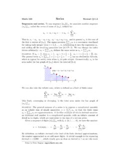
Math 133 Series Sequences and series. fa g
users.math.msu.eduGeometric sequences and series. A general geometric sequence starts with an initial value a 1 = c, and subsequent terms are multiplied by the ratio r, so that a n = ra n 1; explicitly, a n = crn 1. The same trick as above gives a formula for the corresponding geometric series. We have s …
The Laplace Transform (Sect. 6.1). - users.math.msu.edu
users.math.msu.eduThe Laplace Transform (Sect. 6.1). I The definition of the Laplace Transform. I Review: Improper integrals. I Examples of Laplace Transforms. I A table of Laplace Transforms. I Properties of the Laplace Transform. I Laplace Transform and differential equations.
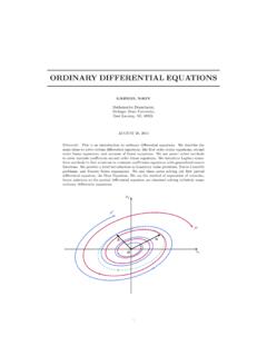
ORDINARY DIFFERENTIAL EQUATIONS
users.math.msu.eduThe equations in examples (c) and (d) are called partial di erential equations (PDE), since the unknown function depends on two or more independent variables, t, x, y, and zin these examples, and their partial derivatives appear in the equations.
Sequences and Series - Michigan State University
users.math.msu.edu2 2. Sequences and Series A topological way to say lima n = ais the following: Given any -neighborhood V (a) of a, there exists a place in the sequence after which all of the terms are in V (a): Easy Fact: lim(c) = cfor all constant sequences (c): Quanti ers. The de nition of lima n = aquanti es the closeness of a n to aby an arbi-
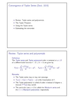
Convergence of Taylor Series (Sect. 10.9) Review: Taylor ...
users.math.msu.eduConvergence of Taylor Series (Sect. 10.9) I Review: Taylor series and polynomials. I The Taylor Theorem. I Using the Taylor series. I Estimating the remainder. The Taylor Theorem Remark: The Taylor polynomial and Taylor series are obtained from a generalization of the Mean Value Theorem: If f : [a,b] → R is differentiable, then there exits c ∈ (a,b) such that
Related documents
Chapter 5: JOINT PROBABILITY DISTRIBUTIONS Part 1 ...
homepage.stat.uiowa.eduGiven random variables Xand Y with joint probability fXY(x;y), the conditional probability distribution of Y given X= xis f Yjx(y) = fXY(x;y) fX(x) for fX(x) >0. The conditional probability can be stated as the joint probability over the marginal probability. Note: we can de ne f Xjy(x) in a similar manner if we are interested in that ...

Notes on Probability
www.maths.qmul.ac.ukHere are the course lecture notes for the course MAS108, Probability I, at Queen ... Joint distributions. Independence. Expectations. Mean, ... In our example, both A and B have probability 4/8=1/2. An event is simple if it consists of just a single outcome, and is compound
Probability, Statistics, and Stochastic Processes
ramanujan.math.trinity.educhapters develop probability theory and introduce the axioms of probability, random variables, and joint distributions. The following two chapters are shorter and of an “introduction to” nature: Chapter 4 on limit theorems and Ch apter 5 on simulation. Statistical inference is treated in Chapter 6, which includes a section on Bayesian v

Topic 7: Random Processes
www.ece.tufts.eduES150 { Harvard SEAS 4. ... † Their joint behavior is completely specifled by the joint distributions for all combinations of their time samples. ... Xn = §1 with probability 1 2 for n even Xn = ¡1=3 and 3 with probabilities 9 10 and 1 10 for n odd † Properties of a WSS process:

Lecture 13 Time Series: Stationarity, AR(p) & MA(q)
www.bauer.uh.edu(4) Forecast. • In this lecture, we go over the statistical theory (stationarity, ... To get asymptotic distributions, we also need a CLT for dependent variables, using the concept of mixing and stationarity. Or we can rely on the martingale CLT. RS –EC2 -Lecture 13 4 • Consider the joint probability distribution of the collection of RVs ...

Lecture 7 Asymptotics of OLS - Bauer College of Business
www.bauer.uh.eduRS – Lecture 7 3 Probability Limit: Convergence in probability • Definition: Convergence in probability Let θbe a constant, ε> 0, and n be the index of the sequence of RV xn.If limn→∞Prob[|xn – θ|> ε] = 0 for any ε> 0, we say that xn converges in probabilityto θ. That is, the probability that the difference between xn and θis larger than any ε>0 goes to zero as n …
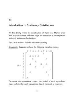
13 Introduction to Stationary Distributions
mast.queensu.catransition probability p ijbeside the directed edge between nodes iand jif p ij >0. For example, here is the state transition diagram for the previous example. 4 3 2 6 1 7 10 9 5 8 1 1 1 1 1 0.9 0.1 0.3 0.3 0.4 0.3 0.3 0.1 0.3 0.2 0.8 0.4 0.6 Figure 13.1: State Transition Diagram for Preceding Example Since the diagram displays all one-step ...

Lecture 1: Entropy and mutual information
www.ece.tufts.eduDefinition The mutual information between two continuous random variables X,Y with joint p.d.f f(x,y) is given by I(X;Y) = ZZ f(x,y)log f(x,y) f(x)f(y) dxdy. (26) For two variables it is possible to represent the different entropic quantities with an analogy to set theory. In Figure 4 we see the different quantities, and how the mutual ...

Lecture 9: Hidden Markov Models
www.cs.mcgill.cat(4) 0.0 0.25 0.0000 0.01562 0.00000 0.00098 0.00049 0.00037 0.00000 0.00000 t(5) 0.0 0.00 0.0625 0.00000 0.00391 0.00000 0.00000 0.00000 0.00009 0.00007 Note that probabilities decrease with the length of the sequence This is due to the fact that we are looking at a joint probability; this phenomenon would not happen for conditional probabilities
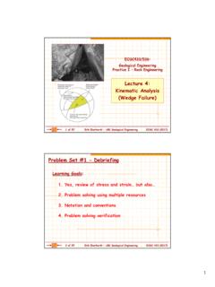
Lecture 4: Kinematic Analysis (Wedge Failure)
www.eoas.ubc.caDiscontinuity Data - Probability Distributions From this, the probability that a given value will be less than dimension x is given by: For example, for a discontinuity set with a mean spacing of 2 m, the probabilities that the spacing will be less than: 1 m 5 m Negative exponential Wyllie & Mah (2004) function: