NUMERICAL STABILITY; IMPLICIT METHODS

THE SECANT METHOD - University of Iowa

THE SECANT METHOD Newton’s method was based on using the line tangent to the curve of y = f(x), with the point of tangency (x 0;f(x 0)).When x 0 ˇ , the graph of the tangent line is approximately the same as the

  Methods, Ascent, The secant method

NUMERICALSOLUTIONOF ORDINARYDIFFERENTIAL …

The differential equations we consider in most of the book are of the form Y′(t) = f(t,Y(t)), where Y(t) is an unknown function that is being sought. The given function f(t,y) of two variables defines the differential equation, and exam ples are given in Chapter 1. This equation is called a first-order differential equation because it ...

  Differential

Lecture 1: The Euler characteristic

7 vertices, 9 edges, 2 faces. We wish to count: 3 vertices, 3 edges, 1 face. 6 vertices, 9 edges, 4 faces. Euler characteristic (simple form): = number of vertices – number of edges + number of faces Or in short-hand, = |V| - |E| + |F| where V = set of vertices E = set of edges ...

  Lecture, Characteristics, Vertices, Euler, Lecture 1, The euler characteristic

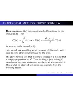
TRAPEZOIDAL METHOD: ERROR FORMULA

The corrected trapezoidal rule is illustrated in the following table. n I T n Ratio I CT n Ratio 2 5.319 3.552E 1 4 1.266 4.20 2.474E 2 14.4 8 3.118E 1 4.06 1.583E 3 15.6

  Rules

ERROR IN LINEAR INTERPOLATION

For f(x) = log 10 x, with 1 x 0 x x 2 10; this leads to jlog 10 x P 2(x)j h3 9 p 3 max x0 x x2 2log 10 e x3:05572h3 x3 0 For the case of h = :01, we have jlog 10 x P 2(x)j 5:57 10 8 x3 0 5:57 10 8 For comparison, jlog 10 x P 1(x)j 5:43 10 6

A quick example calculating the column space and the ...

Put A into echelon form and then into reduced echelon form: R 2 –R 1 R 2 R 3 + 2R 1 R 3 R 1 + 5R 2 R 1 R 2 /2 R 2 R 1 + 8R 3 ...

  Example, Quick, Reduced, Calculating, Space, Columns, Echelon, Quick example calculating the column space and, Reduced echelon

Chapter 5: Numerical Integration and Differentiation

The trapezoidal rule is equivalent to approximating the area of the trapezoidal Figure 1: Graphical depiction of the trapezoidal rule under the straight line connecting f(a) and f(b). An estimate for the local trun-2

  Rules, Trapezoidal, Trapezoidal rule

Different Types of Membership Functions

o Trapezoidal membership function: trapmf. Two membership functions are built on the Gaussian distribution curve: a simple Gaussian curve and a two-sided composite of two different Gaussian curves. The two functions are gaussmf and gauss2mf. The generalized bell membership function is specified by three

  Trapezoidal

Integration Rules and Techniques - Grove City College

Simpson’s Rule (Quadratic Approximation): Uses a quadratic to approximate the function at the top of the \rectangle" over the corresponding subinterval. Zb a f(x) dxˇS n = x 3 ... T be the errors in the Midpoint and Trapezoidal Approximations, respectively. If jf00(x)j K; a x b then jE Mj K(b a)3 24n2 and jE T j K(b a)3 12n2: Let E

  Rules, Technique, Integration, Trapezoidal, Integration rules and techniques

3 Runge-Kutta Methods - IIT

predictor for the (implicit) trapezoidal rule. We obtain general explicit second-order Runge-Kutta methods by assuming y(t+h) = y(t)+h h b 1k˜ 1 +b 2k˜ 2 i +O(h3) (45) with k˜ 1 = f(t,y) k˜ 2 = f(t+c 2h,y +ha 21k˜ 1). Clearly, this is a generalization of the classical Runge-Kutta method since the choice b 1 = b 2 = 1 2 and c 2 = a 21 = 1 ...

  Rules, Trapezoidal, Trapezoidal rule

TRAPEZOIDAL METHOD: ERROR FORMULA

The corrected trapezoidal rule In general, I(f) T n(f) ˇ h2 12 f0(b) f0(a) I(f) ˇCT n(f) := T n(f) h2 12 f0(b) f0(a) This is the corrected trapezoidal rule. It is easy to obtain from the trapezoidal rule, and in most cases, it converges more rapidly than the trapezoidal rule.

  Rules, Trapezoidal, Trapezoidal rule

simpson's 1/3 rule - MATH FOR COLLEGE

The trapezoidal rule was based on approximating the integrand by a first order polynomial, and then integrating the polynomial interval of integration. Simpson’s 1/3 rule is an . over . 07.03.2 Chapter 07.03 . extension of Trapezoidal rule where the integpproximated by a …

  Rules, Trapezoidal, Simpsons, Trapezoidal rule

Romberg Integration - USM

is approximated using the Composite Trapezoidal Rule with step sizes h k = (b a)2 k, where k is a nonnegative integer. Then, for each k, Richardson extrapolation is used k 1 times to previously computed approximations in order to improve the order of accuracy as much as possible.

  Rules, Integration, Trapezoidal, Romberg, Trapezoidal rule, Romberg integration

Chapter 07.02 Trapezoidal Rule of Integration

Trapezoidal Rule of Integration . After reading this chapter, you should be able to: 1. derive the trapezoidal rule of integration, 2. use the trapezoidal rule of integration to solve problems, 3. derive the multiple-segment trapezoidal rule of integration, 4. use the multiple-segment trapezoidal rule of integration to solve problems, and 5.

  Rules, Trapezoidal, Trapezoidal rule

SUGI 27: Using a Trapezoidal Rule for the Area under a ...

The trapezoidal rule is a numerical integration method to be used to approximate the integral or the area under a curve. The integration of [a, b] from a functional form is divided into n equal pieces, called a trapezoid. Each subinterval is approximated by the integrand of a

  Rules, Area, Under, Trapezoidal, Trapezoidal rule, Area under