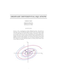
ORDINARY DIFFERENTIAL EQUATIONS

Thomas Calculus; 12th Edition: The Power Rule

Thomas Calculus; 12th Edition: The Power Rule Cli ord E. Weil September 15, 2010 The following paragraph appears at the bottom of page 116 of Thomas Calculus, 12th Edition. The Power Rule is actually valid for all real numbers n.

  Power, Edition, Thomas, Calculus, The power, 12th, Thomas calculus 12th edition, 12th edition, Thomas calculus

Convolution solutions (Sect. 6.6). - users.math.msu.edu

Convolution solutions (Sect. 6.6). I Convolution of two functions. I Properties of convolutions. I Laplace Transform of a convolution. I Impulse response solution. I Solution decomposition theorem.

Special Second Order Equations (Sect. 2.2). Special Second ...

Special Second Order Equations (Sect. 2.2). I Special Second order nonlinear equations. I Function y missing. (Simpler) I Variable t missing. (Harder) I Reduction order method. Special Second order nonlinear equations Definition Given a functions f : R3 → R, a second order differential equation in the unknown function y : R → R is given by

  Second, Special, Order, Equations, Sect, Second order, Special second order equations, Special second order

second order equations{Undetermined Coe - cients

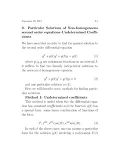
September 29, 2013 9-1 9. Particular Solutions of Non-homogeneous second order equations{Undetermined Coe -cients We have seen that in order to nd the general solution to

  Second, Order, Equations, Undetermined, Second order equations undetermined

5.1 The Remainder and Factor Theorems.doc; Synthetic Division

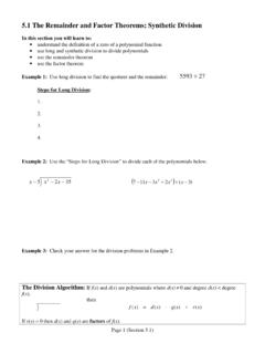
Page 2 (Section 5.1) Example 4: Perform the operation below. Write the remainder as a rational expression (remainder/divisor). 2 1 2 8 2 3 5 4 3 2 + − + + x x x x x Synthetic Division – Generally used for “short” division of polynomials when the divisor is in the form x – c. (Refer to page 506 in your textbook for more examples.)

  Factors, Theorem, Remainder, The remainder and factor theorems

Math 133 Series Sequences and series. fa g

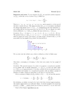
Geometric sequences and series. A general geometric sequence starts with an initial value a 1 = c, and subsequent terms are multiplied by the ratio r, so that a n = ra n 1; explicitly, a n = crn 1. The same trick as above gives a formula for the corresponding geometric series. We have s …

  Series, Sequence, Geometric, Geometric sequences and series, Geometric series, Series sequences and series

The Laplace Transform (Sect. 6.1). - users.math.msu.edu

The Laplace Transform (Sect. 6.1). I The definition of the Laplace Transform. I Review: Improper integrals. I Examples of Laplace Transforms. I A table of Laplace Transforms. I Properties of the Laplace Transform. I Laplace Transform and differential equations.

  Transform, Laplace transforms, Laplace, The laplace transform

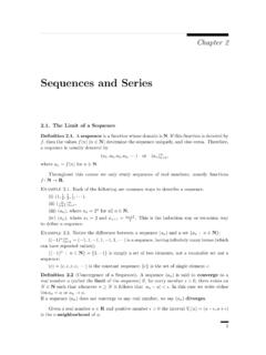
Sequences and Series - Michigan State University

2 2. Sequences and Series A topological way to say lima n = ais the following: Given any -neighborhood V (a) of a, there exists a place in the sequence after which all of the terms are in V (a): Easy Fact: lim(c) = cfor all constant sequences (c): Quanti ers. The de nition of lima n = aquanti es the closeness of a n to aby an arbi-

  Series, Sequence, Sequences and series

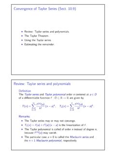
Convergence of Taylor Series (Sect. 10.9) Review: Taylor ...

Convergence of Taylor Series (Sect. 10.9) I Review: Taylor series and polynomials. I The Taylor Theorem. I Using the Taylor series. I Estimating the remainder. The Taylor Theorem Remark: The Taylor polynomial and Taylor series are obtained from a generalization of the Mean Value Theorem: If f : [a,b] → R is differentiable, then there exits c ∈ (a,b) such that

  Review, Convergence

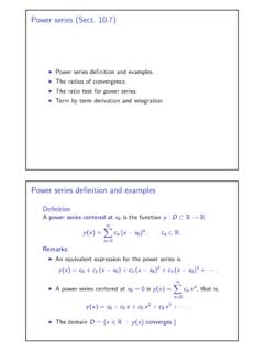
Power series (Sect. 10.7) Power series definition and examples

Power series (Sect. 10.7) I Power series definition and examples. I The radius of convergence. I The ratio test for power series. I Term by term derivation and integration. Power series definition and examples Definition A power series centered at x 0 is the function y : D ⊂ R → R y(x) = X∞ n=0 c n (x − x 0)n, c n ∈ R. Remarks: I An equivalent expression for the power series is

  Series

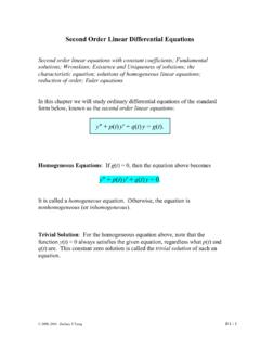
Second Order Linear Differential Equations

reduction of order; Euler equations In this chapter we will study ordinary differential equations of the standard form below, known as the second order linear equations: y″ + p(t) y′ + q(t) y = g(t). Homogeneous Equations: If g(t) = 0, then the equation above becomes y″ + p(t) y′ + q(t) y = 0. It is called a homogeneous equation ...

  Equations, Homogeneous, Homogeneous equations

Lecture 5: Homogeneous Equations and Properties of Matrices

A system of linear equations is said to be homogeneous if the right hand side of each equation is zero, i.e., each equation in the system has the form a 1x 1 + a 2x 2 + + a nx n = 0: Note that x 1 = x 2 = = x n = 0 is always a solution to a homogeneous system of equations, called the trivial solution. Any other solution is a non-trivial solution.

  Equations, Homogeneous, Homogeneous equations

6.4.9 Solutions to homogeneous systems of linear equations

• If you were to solve the corresponding homogeneous system of linear equations, the constant vector in the solution is zero: Solutions to homogeneous systems of linear equations 11 6 3.9 §· ¨¸ ¨¸ ¨¸©¹ 2 22 1.4 01 0 x xx · ¸ ¸ ¸¹ x 0 0 0 §· ¨¸ ¨¸ ¨¸ ©¹ 2 22 1.4 1 00 x xx · ¸ ¸ ¸ ¹ x Example

  Equations, Homogeneous

PARTIAL DIFFERENTIAL EQUATIONS

The linear equation (1.9) is called homogeneous linear PDE, while the equation Lu= g(x;y) (1.11) is called inhomogeneous linear equation. Notice that if uh is a solution to the homogeneous equation (1.9), and upis a particular solution to the inhomogeneous equation (1.11), then uh+upis also a solution to the inhomogeneous equation (1.11). Indeed

  Equations, Homogeneous

Chapter 2 Ordinary Differential Equations

2.2.4 Homogeneous Equations Homogeneous function Homogeneous equation Reduction to separable equation – substitution Homogeneous functions in Rn 2.2.5 Linear 1st order ODE General solution Solution of IVP 2.2.6 Special Equations Bernoulli Equation Ricatti equation Clairaut equation Lagrange equation Equations solvable for y

  Equations, Homogeneous, Homogeneous equations homogeneous

Systems of Differential Equations - University of Utah

The system is called homogeneous if all fj = 0, otherwise it is called non-homogeneous. Matrix Notation for Systems. A non-homogeneous system of ... 526 Systems of Differential Equations corresponding homogeneous system has an equilibrium solution x1(t) = x2(t) = x3(t) = 120. This constant solution is the limit at infinity of

  Equations, Homogeneous

Chapter 7 First-order Differential Equations

Learn to solve typical first order ordinary differential equations of both homogeneous and non‐homogeneous types with or without specified conditions. Learn the definitions of essential physical quantities in fluid mechanics analyses. Learn the Bernoulli’s equation relating the driving pressure and the velocities of ...

  Equations, Homogeneous

Higher Order Linear Differential Equations

Homogeneous equations The general solution If we have a homogeneous linear di erential equation Ly = 0; its solution set will coincide with Ker(L). In particular, the kernel of a linear transformation is a subspace of its domain. Theorem The set of solutions to a linear di erential equation of order n is a subspace of Cn(I). It is called the ...

  Higher, Linear, Order, Equations, Homogeneous, Homogeneous equations, Higher order linear