The Gauss-Jordan Elimination Algorithm

STAT697F - TOPICS IN REGRESSION. REFERENCES

STAT697F - TOPICS IN REGRESSION. REFERENCES Bates and Watts. Nonlinear Regression Analysis. Buonaccorsi (1998) ”Fieller’s Theorem”. Encyclopedia of Biostatistics.

  Reference, Topics, Regression, Stat697f topics in regression, Stat697f

[Chapter 5. Multivariate Probability Distributions]

[Chapter 5. Multivariate Probability Distributions] 5.1 Introduction 5.2 Bivariate and Multivariate probability dis-tributions 5.3 Marginal and Conditional probability dis-tributions 5.4 Independent random variables 5.5 The expected value of a function of ran-dom variables 5.6 Special theorems

  Chapter, Distribution, Probability, Chapter 5, Multivariate, Multivariate probability, Multivariate probability distributions

Matrix-Vector Products and the Matrix Equation Ax= b

Matrices Acting on Vectors The equation Ax = b Geometry of Lines and Planes in R3 Returning to Systems A Proposition on Existence of Solutions Proposition Let A be an m n matrix. Then the following statements are equivalent: For every b 2Rm, the system Ax = b has a solution, Each b 2Rm is a linear combination of the columns of A,

  Product, Equations, Matrix, Panels, Vector, Existence, Matrix vector products and the matrix equation

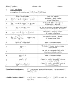
I. The Limit Laws

Math131 Calculus I Limits at Infinity & Horizontal Asymptotes Notes 2.6 Definitions of Limits at Large Numbers Theorem • If r > 0 is a rational number then 0 1 lim = x →∞ xr • If r > 0 is a rational number such that xr is defined for all x then 0 1

  Limits, Theorem

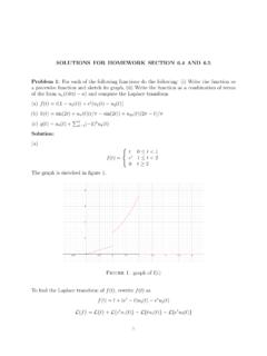
SOLUTIONS FOR HOMEWORK SECTION 6.4 AND 6.5 Problem 1

The inverse Laplace transform of H(s) is h(t) = L1fHg= 1 6 (1 e 6t) Hence, by using t-shifting theorem if necessary, we can nd the solution y(t) = LfYg= 12u ... Hint: Rewrite costusing a trigonometric identity. Solution: First need to write u ˇ=2(t)costin the form u c(t)f(t c). To do this use the trig identities

  Inverse, Trigonometric

The mathematics of cryptology

1881 9881292060 7963838697 2394616504 3980716356 3379417382 7007633564 2298885971 5234665485 3190606065 0474304531 7388011303 3967161996 9232120573 4031879550 6569962213 0516875930 7650257059 into its two 87-digit prime factors. For this they won the not too shabby sum of $10,000. Such “challenges” are the only way we know that RSA is ...

  1881

Polar Coordinates (r,θ

Polar Coordinates (r,θ) Polar Coordinates (r,θ) in the plane are described by r = distance from the origin and θ ∈ [0,2π) is the counter-clockwise angle.

  Coordinates, Panels, Polar, Polar coordinates

Limits and Continuity for Multivariate Functions

A. Havens Limits and Continuity for Multivariate Functions. De ning Limits of Two Variable functions Case Studies in Two Dimensions Continuity Three or more Variables An Epsilon-Delta Game Epsilong Proofs: When’s the punchline? Since 3 times this distance is an upper bound for jf(x;y) 0j, we simply choose to ensure 3 p

  Continuity, Limits, Limits and continuity

OpenMP by Example

To build one of the examples, type ”make <EXAMPLE.X>” (where <EXAMPLE> is the name of file you want to build (e.g. make test.x will compile a file test.f).

  Example, Openmp

Multivariate Functions and Partial Derivatives

2/21/20 Multivariate Calculus: Multivariable Functions Havens Figure 1. The graph of the paraboloid given by z= f(x;y) = 4 1 4 (x 2 + y2). Vertical trace curves form …

  Functions, Partial, Derivatives, Functions and partial derivatives

CHAPTER 8: MATRICES and DETERMINANTS

Coefficient matrix Right-hand side (RHS) Augmented matrix We may refer to the first three columns as the x-column, the y-column, and the z-column of the coefficient matrix. Warning: If you do not insert “1”s and “0”s, you may want to read the equations and fill out the matrix row by row in order to minimize the chance of errors.

  Determinants, Chapter, Equations, Matrix, Chapter 8, Three, Matrices and determinants, Matrices

Linear Algebra in Twenty Five Lectures

Linear Algebra in Twenty Five Lectures Tom Denton and Andrew Waldron March 27, 2012 Edited by Katrina Glaeser, Rohit Thomas & Travis Scrimshaw 1

A SAMPLE RESEARCH PAPER/THESIS/DISSERTATION ON …

Theorem 1.2.1. A homogenous system of linear equations with more unknowns than equations always has infinitely many solutions The definition of matrix multiplication requires that the number of columns of the first factor A be the same as the number of rows …

  Equations, Matrix, Thesis

Expected Value and Markov Chains - aquatutoring.org

The matrix N= (I Q) 1 is called the fundamental matrix for P. The entry n ij of Ngives the expected number of times that the process is in the transient state jif it started in the transient state i. (See [1] for a proof.) Since I Q= 0 @ 1 1 0 1=5 3=5 2=5 0 2=5 3=5 1 A; we can use Gauss-Jordan elimination to calculate its inverse matrix and get ...

  Chain, Value, Expected, Matrix, Elimination, Markov, Expected value and markov chains

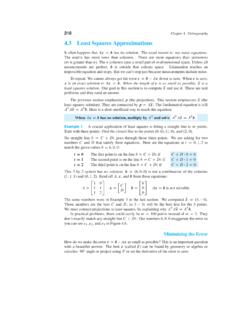
4.3 Least Squares Approximations - MIT Mathematics

of bx. The equations from calculus are the same as the “normal equations” from linear algebra. These are the key equations of least squares: The partial derivatives of kAx bk2 are zero when ATAbx DATb: The solution is C D5 and D D3. Therefore b D5 3t is the best line—it comes closest to the three points. At t D0, 1, 2 this line goes ...

  Tesla, Square, Equations, Three, Least squares

Nodal and Loop Analysis - Waterloo Maple

This can be solved easily as a matrix with Maple using the solve command. Otherwise, use substitution and elimination with the KCL equations to solve for the values of the node voltages. = Thus the potential of the node voltages are , and . MapleSim Solution Step 1: Insert Components Drag the following components into a new workspace.

  Equations, Matrix, Elimination, Solve, Equations to solve

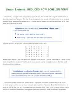
Linear Systems: REDUCED ROW ECHELON FORM

semester progresses because so many concepts and properties of a matrix can then be described in terms of . But first let's investigate how the presence of the 1 and 0's in the pivot column affects the Gauss Elimination method for solving three particular systems of linear equations in 3 variables. A A A 1 1! " ## ## ## # 1 0 0 0 0 0 ∗ 0 0 0 ...

  Equations, Matrix, Three, Elimination

2.5 Inverse Matrices - MIT Mathematics

84 Chapter 2. Solving Linear Equations The Gauss-Jordan method computes A 1 by solving all n equations together. Usually the “augmented matrix” ŒA b has one extra column b. Now we have three right sides e1;e2;e3 (when A is 3 by 3). They are the columns of I, so the augmented

  Equations, Matrix, Three

2.5 Inverse Matrices - MIT Mathematics

To invert a 3 by 3 matrix A, we have to solve three systems of equations: Ax 1 = e 1 and Ax 2 = e 2 = (0,1,0) and Ax 3 = e 3 = (0,0,1). Gauss-Jordan finds A−1 this way. The Gauss-Jordan method computesA−1 by solving all n equations together. Usually the “augmented matrix” [A b] has one extra column b. Now we have three right sides e 1 ...

  Equations, Matrix, Three, Solve, Inverse, To solve three

Finding the Dimension and Basis of the Image and Kernel of ...

So, to nd out which columns of a matrix are independent and which ones are redundant, we will set up the equation c 1v 1 + c 2v 2 + :::+ c nv n = 0, where v i is the ith column of the matrix and see if we can make any relations. ex. Consider the matrix 0 B B @ 1 3 1 4 2 7 3 9 1 5 3 1 1 2 0 8 1 C C A which de nes a linear transformation from R4 ...

  Dimensions, Matrix