Transcription of Solutions for Tutorial 3 Modelling of Dynamic Systems
1 McMaster University 11/05/05 Copyright 2000 by T. Marlin 1 Solutions for Tutorial 3 Modelling of Dynamic Systems Mixer: Dynamic model of a CSTR is derived in textbook Example From the model, we know that the outlet concentration of A, CA, can be affected by manipulating the feed concentration, CA0, because there is a causal relationship between these variables. a. The feed concentration, CA0, results from mixing a stream of pure A with solvent, as shown in the diagram. The desired value of CA0 can be achieved by adding a right amount of A in the solvent stream. Determine the model that relates the flow rate of reactant A, FA, and the feed concentration, CA0, at constant solvent flow rate. b. Relate the gain and time constant(s) to parameters in the process. c. Describe a control valve that could be used to affect the flow of component A.
2 Describe the a) valve body and b) method for changing its percent opening (actuator). Figure a. In this question, we are interested in the behavior at the mixing point, which is identified by the red circle in the figure above. We will apply the standard Modelling approach to this question. Goal: Determine the behavior of CA0(t) System: The liquid in the mixing point. (We assume that the mixing occurs essentially immediately at the point.) SolventReactantFoCAOF1 CAFsCA,solventFACA,reactantMcMaster University 11/05/05 Copyright 2000 by T. Marlin 2 Balance: Since we seek the behavior of a composition, we begin with a component balance. Accumulation = in - out + generation (1) ()()0)CFF(CFCFtMX|CV|CVMW0 AASAAAASSAt0 Amtt0 AmA++ + = + Note that no reaction occurs at the mixing point.
3 We cancel the molecular weight, divide by the delta time, and take the limit to yield (2) 0 AAAASAASASSAASmCCFFFCFFFdtdC)FF(V +++=+ No reactant (A) appears in the solvent, and the volume of the mixing point is very small. Therefore, the model simplifies to the following algebraic form. (3) 0 AAAASACCFFF=+ Are we done? We can check degrees of freedom. DOF = 1 1 = 0 Therefore, the model is complete. CA0 (FS, FA, and CAA are known) You developed models similar to equation (3) in your first course in Chemical Engineering, Material and Energy balances. (See Felder and Rousseau for a refresher.) We see that the Dynamic Modelling method yields a steady-state model when the time derivative is zero. Note that if the flow of solvent is much larger than the flow of reactant, FS >> FA, then, (4) ASAA0AF FCC = If FS and CAA (concentration of pure reactant) are constant, the concentration of the mixed stream is linearly dependent on the flow of reactant.
4 B. For the result in equation (4), Time constant = 0 (This is a steady-state process.) Gain = CAA/FS (The value will change as FS is changed.) McMaster University 11/05/05 Copyright 2000 by T. Marlin 3 c. The control valve should have the following capabilities. 1. Introduce a restriction to flow. 2. Allow the restriction to be changed. 3. Have a method for automatic adjustment of the restriction, not requiring intervention by a human. 1&2 These are typically achieved by placing an adjustable element near a restriction through which the fluid must flow. As the element s position in changed, the area through which the fluid flows can be increased or decreased. 3 This requirement is typically achieved by connecting the adjustable element to a metal rod (stem). The position of the rod can be changed to achieve the required restriction.
5 The power source for moving the rod is usually air pressure, because it is safe (no sparks) and reliable. A rough schematic of an automatic control valve is given in the following figure. See a Valve You can see a picture of a typical control valve by clicking here. Many other valves are used, but this picture shows you the key features of a real, industrial control valve. Hint: To return to this current page after seeing the valve, click on the previous view arrow on the Adobe toolbar. You can read more about valves at the McMaster WEB site. air pressurevalve stem positiondiaphramspringvalve plug and seatMcMaster University 11/05/05 Copyright 2000 by T. Marlin 4 Stirred tank mixer a. Determine the Dynamic response of the tank temperature, T, to a step change in the inlet temperature, T0, for the continuous stirred tank shown in the Figure below.
6 B. Sketch the Dynamic behavior of T(t). c. Relate the gain and time constants to the process parameters. d. Select a temperature sensor that gives accuracy better than 1 K at a temperature of 200 K. Figure We note that this question is a simpler version of the stirred tank heat exchanger in textbook Example Perhaps, this simple example will help us in understanding the heat exchanger example, which has no new principles, but more complex algebraic manipulations. Remember, we use heat exchangers often, so we need to understand their Dynamic behavior. a/c. The Dynamic model is derived using the standard Modelling steps. Goal: The temperature in the stirred tank. System: The liquid in the tank. See the figure above. Balance: Since we seek the temperature, we begin with an energy balance. FT0 TVFMcMaster University 11/05/05 Copyright 2000 by T.
7 Marlin 5 Before writing the balance, we note that the kinetic and potential energies of the accumulation, in flow and out flow do not change. Also, the volume in the tank is essentially constant, because of the overflow design of the tank. accumulation = in - out (no accumulation!) (1) ())HH(t|U|Uoutinttt = + We divide by delta time and take the limit. (2) )HH(dtdUoutin = The following thermodynamic relationships are used to relate the system energy to the temperature. dU/dt = V Cv dT/dt H = F Cp (T-Tref) For this liquid system, Cv Cp Substituting gives the following. (3) )TT(FdtdTV0 = Are we done? Let s check the degrees of freedom. DOF = 1 1 = 0 T (V, and T0 known) This equation can be rearranged and subtracted from its initial steady state to give (4) 0'KT'Tdt'dT=+ with = V/F K = 1 Note that the time constant is V/F and the gain is These are not always true!
8 We must derive the models to determine the relationship between the process and the dynamics. See Example for different results for the stirred tank heat exchanger. McMaster University 11/05/05 Copyright 2000 by T. Marlin 6 The Dynamic response for the first order equation differential equation to a step in inlet temperature can be derived in the same manner as in Examples , , etc. The result is the following expression . (5) )e1(TK'T/t0 = and )e1(TK TT/t0initial += d. We base the temperature sensor selection on the information on advantages and disadvantages of sensors. A table is available on the McMaster WEB site, and links are provided to more extensive sensor information. A version of such a table is given below. Since a high accuracy is required for a temperature around 200 K, an RTD (a sensor based on the temperature sensitivity of electrical resistance) is recommended.
9 Even this choice might not achieve the 1 K accuracy requirement. sensor type limits of application ( C) accuracy (1,2) dynamics, time constant (s) advantages disadvantages thermocouple type E (chromel-constantan) type J (iron-constantan) type K (chromel-nickel) type T (copper-constantan) -100 to 1000 0 to 750 0 to 1250 -160 to 400 or (0 to 900 C) or or or (-160 to 0 C) (3) 1. good reproducibility 2. wide range 1. minimum span, 40 C 2. temperature vs emf not exactly linear 3. drift over time 4. low emf corrupted by noise RTD -200 to 650 ( +.02 T ) C (3) 1. good accuracy 2. small span possible 3. linearity 1. self heating 2. less physically rugged 3. self-heating error Thermister -40 to 150 C (3) 1. good accuracy 2. little drift 1.
10 Highly nonlinear 2. only small span 3. less physically rugged 4. drift Bimetallic 2% 1. low cost 2. physically rugged 1. local display Filled system -200 to 800 1% 1-10 1. simple and low cost 2. no hazards 1. not high temperatures 2. sensitive to external pressure 1. C or % of span, whichever is larger 2. for RTDs, inaccuracy increases approximately linearly with temperature deviation from 0 C 3. dynamics depend strongly on the sheath or thermowell (material, diameter and wall thickness), location of element in the sheath ( , bonded or air space), fluid type, and fluid velocity. Typical values are 2-5 seconds for high fluid velocities. TimeTimeTT0 McMaster University 11/05/05 Copyright 2000 by T. Marlin 7 Isothermal CSTR: The model used to predict the concentration of the product, CB, in an isothermal CSTR will be formulated in this exercise.