Transcription of Chapter 8 More Discrete Probability Models
1 Chapter 8 more Discrete Probability IntroductionIn the previous Chapter we started to look at Discrete Probability Models . This week we lookat two of the most common Models for Discrete data: the binomial distribution and the The Binomial DistributionIn many surveys and experiments data is collected in the formof counts. For example, thenumber of people in the survey who bought a CD in the past month, the number of people whosaid they would vote Labour at the next election, the number of defective items in a sampletaken from a production line, and so on.
2 All these variables have common features:1. Each person/item has only two possible responses or outcomes (Yes/No, Defective/Notdefective etc) this is referred to as atrialwhich results in The survey/experiment takes the form of a random sample the responses The Probability of a success in each trial isp(in which case the Probability of a failure is1 p).4. We are interested in the random variableX, the total number of successes out these conditions are met thenXhas abinomial distributionwith indexnand write this asX Bin(n, p), which reads as Xhas a binomial distribution with indexnand probabilityp.
3 Here,nandpare known as the parameters of the binomial the dice rolling example from Chapter 7. We were interested in the number of sixesobtained from three rolls of a 6-sided die. Treating each roll of the die as atrial, with a sixrepresenting asuccessand not a six representing afailure, we can see that we haven= 3independent trials, each with Probability of successp= 1/6. Thus ifXrepresents the number81 Chapter 8. more Discrete Probability MODELS82of sixes on the 3 rolls, we have thatXhas a binomial distribution with parametersn= 3andp= 1/6, that isX Bin(3,1/6).
4 Probability calculationsHow can we work out probabilities from a binomial distribution? For example, what isP(X=2)in the dice rolling example? Well, as was mentioned in Chapter 7, there is a formula thatallows us to work out such probabilities for any values ofnandp. The Probability thatXtakes the valuer, that is, that there arersuccesses out ofntrials, can be calculated using thefollowing formula:P(X=r) =(# ways to getrsuccesses out ofntrials) P(rsuccesses) P(n rfailures)=nCr pr (1 p)n r,r= 0,1, .. , n,wherenCris the number of combinations ofrobjects out ofn(see Section , page 75),pisthe Probability of success, and(1 p)is the Probability of failure, on a single trial.
5 Recall thatnCr=n!r!(n r)!, and there is a button on most scientific calculators to compute this directly. Notethat any number raised to the power zero is equal to one, for example, Bin(3,1/6), as in the dice rolling example, then P(X= 2) =nCr pr (1 p)n r=3C2 (16)2 (1 16)3 2= 3 (16)2 (56)= exampleA salesperson has a 50% chance of making a sale on a customer visit and she arranges 6 visitsin a day. What are the probabilities of her making 0,1,2,3,4,5 and 6 sales?LetXdenote the number of sales. Assuming the visits result in sales independently, thenX Bin(6, )and using the formula forP(X=r)given above we can compute the following:No.
6 Of sales Probability Cumulative ProbabilityrP(X=r)P(X r) 8. more Discrete Probability MODELS83 The formula for binomial probabilities enables us to calculate values forP(X=r). From these,it is straightforward to calculate cumulative probabilities such as the Probability of making nomore than 2 sales:P(X 2) =P(X= 0) +P(X= 1) +P(X= 2)=6C0(12)0(12)6+6C1(12)1(12)5+6C2(12)2( 12)4= + + cumulative probabilities are also useful in calculating probabilities such as that of makingmore than 1 sale: P(X >1) =1 P(X 1)= 1 ,which uses the fact that the sum of all the probabilities in a Discrete Probability distribution isequal to Mean and varianceIf we have the Probability distribution forXrather than the raw observations, we denote themean forXnot by xbut byE[X](which reads as the expectation ofX ), and the variance byV ar(X).
7 IfXis a random variable with a binomialBin(n, p)distribution then its mean and varianceareE[X] =n p,V ar(X) =n p (1 p).For example, ifX Bin(6, )then E[X] =np= 6 = 3andV ar(X) =np(1 p) = 6 = (X) = V ar(X) = = 8. more Discrete Probability The Poisson DistributionThePoisson distributionis a very important Discrete Probability distribution which arises inmany different contexts. Typically, Poisson random quantities are used in place of binomialrandom quantities in situations wherenis large,pis small, and bothnpandn(1 p)exceed general, it is used to model data which are counts of (random)
8 Events in a certain area or timeinterval, without a known fixed upper limit but with a knownrateof example, consider the number of calls made in a 1 minute interval to a telephone call call centre has thousands of customers, but each one willcall with a very small the call centre knows that on average 5 calls will be made inany 1 minute interval, the actualnumber of calls will be a Poisson random variable, with mean Probability distributionIfXis a random variable with a Poisson distribution with parameter (Greek lower case lambda ) then the Probability it takes different values isP(X=r) = re r!
9 , r= 0,1,2, ..We write this asX P o( ). The parameter has a very simple interpretation as the average,or expected, number of Mean and varianceThe distribution has mean and varianceE[X] = ,V ar(X) = .Thus, when approximating binomial probabilities by Poisson probabilities, we match the meansof the distributions: = to the call centre example, suppose we want to knowthe probabilities of differentnumbers of calls made to the call centre. LetXbe the number of calls made in a minute. ThenX P o(5)and, for example, the Probability of receiving 4 calls is P(X= 4) =54e 54!
10 = can use the formula for Poisson probabilities to calculate the Probability of all possibleoutcomes: Chapter 8. more Discrete Probability MODELS85 Probability Cumulative ProbabilityrP(X=r)P(X r) the Probability of receiving between 2 and 8 callsisP(2 X 8) =P(X 8) P(X 1) = = so is very calculations such as this enable the call centre to forecast the likely demand fortheir service and hence the resources they need to provide the service. Using such a model wecan also account for extreme situations. For example, suppose that, for this call centre, weobserved the following number of calls per minute over a five minute period: 6, 3, 5, 4, 6.