Statistics 2 - Assets - Cambridge University Press

1 Advanced Level MathematicsStatistics 2 Steve Dobbs and Jane MillerSeries editorHugh NeillPUBLISHED BY THE Press SYNDICATE OF THE University OF CAMBRIDGEThe Pitt Building, Trumpington Street, Cambridge , United KingdomCAMBRIDGE University PRESSThe Edinburgh Building, Cambridge CB2 2RU, UK40 West 20th Street, New York, NY 10011-4211, USA477 Williamstown Road, Port Melbourne, VIC 3207, AustraliaRuiz de Alarc n 13, 28014 Madrid, SpainDock House, The Waterfront, Cape Town 8001, South Cambridge University Press 2000 This book is in copyright. Subject to statutory exceptionand to the provisions of relevant collective licensing agreements,no reproduction of any part may take place withoutthe written permission of Cambridge University published 2000 Fourth printing 2002 Printed in the United Kingdo mat the University Press , Ca mbridgeTypefacesTimes, HelveticaSystemsMicrosoft Word, MathType?

2 A catalogue record for this book is available from the British LibraryISBN 0 521 78604 5paperbackCover image: Images Colour LibraryContentsIntroductionvii1 Continuous random variables12 The normal distribution203 ThePoisson distribution484 Sampling685 Hypothesis testing:continuous variables996 Hypothesis testing: discrete variable1177 Errors in hypothesis testing130 Revision exercise151 Mock examinations155 Answers173 Inde x183 Cumulative binomial probabilities161 Cumulative Poisson probabilities168 The normal distribution function1721 Continuous random variablesThis chapter looks at the way in which continuous random variables are modelledmathematically.

3 When you have completed it you should understand what a continuous random variable is know the properties of a probability density function and be able to use them be able to use a probability density function to solve problems involving probabilities be able to find the median of a distribution in simple cases be able to calculate the mean and variance of a Comparing discrete and continuous random variablesIn S1 Section , you met the idea of a random variable and its probability order to refresh your memory, consider the random variable , H, which is the numberof heads obtained when two coins are spun. This random variable can take the values 0,1 and 2 with probabilities of 14, 12 and 14 that you know how these probabilities were notation used to express these results is P=H014()=, P=H112()= andP=H214()=.

4 Alternatively, you can display these results in a table, as in Table of heads, h012P=Hh()141214 Table Probability distribution of H, the number of heads when two coins are random variables which you studied in S1 were all discrete random variables; thatis, there were clear steps between the possible values which the variable could are many variables, however, which are not the following example. The cars on a ski-lift are attached at equal intervalsalong a cable which travels at a fixed speed. The speed of the cars is so low that people canstep in and out of the cars at the station without the cars having to stop.

5 The time intervalbetween one car and the next arriving at the station is 5 minutes. You do not know thetimetable for the cars and so you turn up at the station at a random time and wait for a waiting time, X (measured in minutes), is an example of a random variable becauseits value depends on chance. However, it is also a continuous variable because the waitingtime can take any value in the interval 0 to 5 minutes, that is 05 X<.In S1 in order to describe a discrete random variable completely, you obtained aprobability for each possible value of the random variable . If you try the same approachwith a continuous random variable you run into difficulties: because the waiting time,X, can take an infinite number of values in the interval 0 to 5 minutes, you cannotwrite out a table like Table However, you do know that if you arrive at the station at2 Statistics 2a random time, all values of X are equally likely.

6 Would it be possible to describe thedistribution by stating that all values of X between 0 and 5 are equally likely and byassigning the same non-zero probability to each one? This gives rise to another sum of the probabilities will not be one, as it should be, but will be infinite since Xtakes an infinite number of values. Obviously a different approach is needed in order todescribe the probability distribution of a continuous random variable . This will beconsidered in the next Defining the probability distribution of a continuous random variableAlthough it is not possible to give the probability that X (the waiting time in Section )takes a particular value, it does make sense to talk about X taking a value within a particularrange.

7 For example, you would expect that P02512 X.()= since the interval from 0 to25. accounts for half the values which X can take,and all values are equally likely. Extending this idea,you would expect P0115 X<()= since this intervalcovers 15 of the total interval. SimilarlyP12 X<()=<()=<()PP2334 XX=<()=P45 02 X.. These probabilities could berepresented on a diagram similar to a histogram, asshown in Fig. In this diagram the area of eachblock gives the probability that X lies in thecorresponding interval. Since the width of each blockis 1 its height must be 0 2. in order to make the areaequal to 0 2.. Notice that the total area under the curvemust be one since the probabilities must sum to choice of the intervals 0 to 1, 1 to 2 and so on isarbitrary.

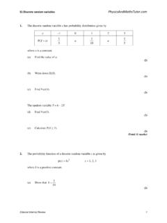
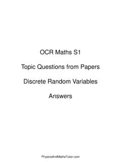
8 In order to make the model more general youneed to be able to find the probability that X lieswithin any given interval. Suppose that the divisionsbetween the blocks in Fig. are removed so as togive Fig. In this diagram, probabilities stillcorrespond to areas. For example, P 0 51.<()X isgiven by the area under the curve between 05. and is shown as the shaded area in Fig. : its valueis 0 1. as you would should now be able to see that the probabilitydistribution of the waiting times can be modelled bythe continuous function fx() which describes Fig. required function isffor ()=< 0250., 012345 Waiting time, x (min) Diagram to represent theprobabilities of waiting times for a time, x (min) Diagram to represent thedistribution of waiting times for a time, x (min) Diagram to represent theprobability of waiting between and for the that it is usual to define fx() for all real values of 1: CONTINUOUS random VARIABLES3 Once fx() has been defined, you can find probabilities by calculating areas below thecurve y= xf().

9 For example, P 1 33 50 23 5 1 30 X()= ()=Notice that, if you want the probability that X=13. or the probability that X=35. , theanswer is zero. These are just single instants of time, and although it is theoretically possiblethat a car may arrive at either of those instants, the probability is actually zero. This meansthat .<<()=<()XX = .<()=()XX . Thissituation is characteristic of continuous function fx() is called a probability density function. It cannot take negative valuesbecause probabilities are never negative. It must also have the property that the total areaunder the curve y= xf() is equal to one.

10 This is because this area represents theprobability that X takes any real value and this probability must be suitability of this function as a model for actual waiting times could be tested bycollecting some data and comparing a histogram of these experimental results with theshape of y= xf(). Some results are given in Table time,x (min)FrequencyRelativefrequencyClass widthRelative frequencydensity01 x< x< x< x< Waiting times for the ski-lift for a sample of 500 third column gives the relativefrequencies: these are found by dividing eachfrequency by the total frequency, in this case500. The relative frequency gives theexperimental probability that the waiting timelies in a given interval.