Transcription of 1 Cobb-Douglas Functions - University of Vermont
1 1 Cobb-Douglas Functions Cobb-Douglas Functions are used for both production Functions Q = K L(1 ). where Q is output, and K is capital and L is labor. The same functional form is also used for the utility function; we often write: U = X Y (1 ). where X and Y are two di erent goods. These two expressions are mathemat- ically equivalent. The Cobb-Douglas function is three dimensional with utility or output mea- sured along the vertical axis. 5. y 5 5. z 0 0. x We rarely work with 3-D graphs such as this however; instead we slice it into various views or projections. The projection onto the XY axis is called an indi erence curve. The projection is made by slicing o the top of the three- dimensional utility surface and shinning a light from above. The shadow that the edge projects on the floor is the indi erence curve.
2 These projections are useful for graphical purposes only; when working with them, we must remember that we are still using the full Cobb-Douglas equation. To get the XY projection in the utility function, we simply take a given level of U = U0 and solve for Y as a function of X. U0 = X Y (1 ). Solution is: 1 . Y = U01 X 1 . 1. but since U01 is a constant along the projection, this is simply an hyperbola. It has a graph that looks like: 1. y 100. 75. 50. 25. 0 5 10 15 20. x which is an indi erence curve, or combinations of X and Y such that the level of utility is a constant, U0 . For U1 > U0 the curve would shift out from the origin, but along the curve, total utility is constant. Indi erence curves are similar to topographical maps; all along an indi erence curve, we are at the same altitude above the floor.
3 The projection in the X, U plane can be also be plotted and studied as in the following figure. To get this graph start with a given level of Y and plot U = X Y (1 ). where the bar over Y indicates that Y is constant. Increasing Y would shift the curve upward. U. 50. 25. 0. 0 25 50. X. and a similar diagram can be drawn for the projection into the Y, U plane. Slopes For the utility function, the slope of this curve in the X, U plane is just the marginal utility of X, holding Y constant. For the production function, the slope is the marginal product of one of the two factors, holding the other con- stant. Using calculus, the slope is simply the partial derivative of the cobb - 2. Douglas function with respect to X holding Y constant, or vice-versa. U. = marginal utility of X. X |Y =Y . One of the reasons the Cobb-Douglas is so popular is that its derivatives are so simple.
4 The function itself is not, but taking the partial of U with respect to X gives: U U. = X 1 Y 1 =. X X. With respect to Y. U (1 )U. = (1 )X Y 1 1 =. Y Y. The slope of the horizontal projection The horizontal projection of the utility function is an indi erence curve. For a production function, it is an isoquant. The slope of either of these two curves in just the rise over the run as it would be in any 2-D space. For the square root version of the Cobb-Douglas , = , the slope is very easy to calculate. Consider an indi erence curve. First pick a point on the curve, call it X1 , Y1 . On the same indi erence curve a second point might be X2 Y2 and think of it has lower and to the right of the first point. The run is just X2 X1 while the rise is Y2 Y1 . But since Y2 is less than Y1 the rise is negative. Since both points are on the indi erence curve, the utility must be the same.
5 We have: U (X1 , Y1 ) = U (X2 , Y2 ). Subtracting, we can write: U12 U22 = 0.. where Ui = Xi , Yi . Finally, rewrite this last equation as: X1 Y1 X2 Y2 = 0. To get the slope of the indi erence curve, we can just add and subtract X1 Y2 to the last equation and write the result as: X1 Y1 X2 Y2 + X1 Y2 X1 Y2 = 0. This is a key substitution, one that only works for the square root version of the Cobb-Douglas . Reorganizing this last expression X1 (Y1 Y2 ) + (X1 X2 )Y2 = 0. The elements a slope, the rise (Y1 Y2 ) over run (X1 X2 ) are starting to take shape. Divide both sides by (X1 X2 ). (Y1 Y2 ). X1 + Y2 = 0. (X1 X2 ). 3. Y. X2Y 2. rise X1Y 1. run X. Figure 1: and call the slope, . X1 + Y2 = 0. Y2. and solve for = X 1. This is the slope of the straight line in the graph above. To get the in- stantaneous slope at the point X1 Y1 , just move the two points closer and closer together, that is move X2 Y2 down toward X1 Y1.
6 In the limit, that is as the distance between the points goes to zero, we have: Y. = . X. The slope is known as the marginal rate of substitution. In the case of the isoquant, the argument is identical; instead of X and Y. we have K and L. But this gives: K. = . L. so long as L is on the horizontal axis, taking the place of X. For the isoquant, the slope is known as the marginal rate of technical substitution. Another way to get slopes of horizontal projections is to use multivariate calculus. It gets the same result, but requires that you understand a total di erential of a function of two variables. In the case of utility, the total di erential of U is: 4. U U. dU = dX + dY. X Y. U. where X is a partial derivative, that is the derivative of U with respect to X holding Y constant, said the partial of U with respect to Y.
7 1 As we saw above, along an indi erence curve or an isoquant, the change in U , dU = 0. We then have: U U. dX +. 0= dY. X Y. from which the slope, dY/dX of the indi erence curve can be calculated. dY U/ X. = . dX U/ Y. but since the partial derivative of the Cobb-Douglas function is just U U. = X 1 Y 1 =. X X. and with respect to Y. U (1 )U. = (1 )X Y 1 1 =. Y Y. we have substituting into the definition of the slope: dY UY Y. = = . dX (1 )U X (1 )X. This is the general expression for the slope of the two-dimensional projection of the the Cobb-Douglas equation into the XY plane. In the special case of the square root function ( = ) we have: dY Y. == . dX X. which is the same as the expression above. Using the Cobb-Douglas for Utility or Profit Maxi- mization Now whether we are talking about maximizing utility or minimizing cost, setting the slope of the 2-D projection is set equal to the slope of the constraint is gives one equation for the solution to the maximization problem.
8 For example, in the maximization of utility problem the slope of the budget constraint is just the (negative of the ) opportunity cost of X in terms of the good U. 1 Similarly, the derivative of U with respect to Y holding X constant is Y.. 5. Y, in other words, pX /pY , the price of X divided by the price of Y. Maximizing utility is requires that these two slopes are the same: Y. = pX /pY. X. This is the tangency condition which must be solved simultaneously with the budget constraint in order to find a maximum: B = pX X + pY Y. where B is the budget. Substituting the tangency condition into the budget constraint for Y , we have: pX. B = pX X + pY ( X). pY. Simplifying: B = 2pX X. X = B/2pX. and finally, substituting X into the budget constraint B = pX (B/2pX ) + pY Y. or simplifying Y = B/2pY. So the solution involves setting dividing the budget into to two shares depending on their prices.
9 Example 1 Solution 2 Problem 3 Problem 4 Let pX = 1 and pY = 2 and B = 10. Solve the consumer's maximization problem. Solution 5 X = B/2pX = 10/[2(1)] = 5; and Y = B/2pY = 10/[2(2)] =. Check to see that the budget is exhausted. Total utility is U = graphical solution is presented below: y 5. 0. 0 5 10. x 6. Example 6 Solution 7 Problem 8 Problem 9 Let w = 1 and r = 2 and C = 6. Solve the producer's maximization problem. Solution 10 To maximize profits relative to a budget constraint we set slope . of the cost constraint C = wL + rK, which is = w/r equal to the slope of the isoquant dK/dL = K/L. and solve simultaneously with the cost constraint itself. The structure of this problem is identical to that of consumer's problem. The are mathematically equivalent. Solving in the same was as in the previous example, L = C/2w =.
10 6/[2(1)] = 3; and K = C/2r = 6/[2(2)] = Check to see that the cost constraint is exhausted. Output is Q = KL = 7.