Transcription of 1 Linear Quadratic Regulator - cds.caltech.edu
1 CALIFORNIA INSTITUTE OF TECHNOLOGY. Control and Dynamical Systems CDS 110b R. M. murray Lecture 2 LQR Control 11 January 2006. This lecture provides a brief derivation of the Linear Quadratic Regulator (LQR) and describes how to design an LQR-based compensator. The use of integral feedback to eliminate steady state error is also described. Two design examples are given: lateral control of the position of a simplified vectored thrust aircraft and speed control for an automobile. 1 Linear Quadratic Regulator The finite horizon, Linear Quadratic Regulator (LQR) is given by x = Ax + Bu x Rn , u Rn , x0 given Z. 1 T T 1. J= x Qx + uT Ru dt + xT (T )P1 x(T ). 2 0 2. where Q 0, R > 0, P1 0 are symmetric, positive (semi-) definite matrices. Note the factor of 12 is left out, but we included it here to simplify the derivation. Gives same answer (with 21 x cost). Solve via maximum principle: H = xT Qx + uT Ru + T (Ax + Bu). T. H. x = = Ax + Bu x(0) = x0.. T. H. = = Qx + AT (T ) = P1 x(T ).
2 X H. 0= = Ru + T B = u = R 1 B T . u This gives the optimal solution. Apply by solving two point boundary value problem (hard). Alternative: guess the form of the solution, (t) = P (t)x(t). Then = P x + P x = P x + P (Ax BR 1 B T P )x P x P Ax + P BR 1 BP x = Qx + AT P x. This equation is satisfied if we can find P (t) such that P = P A + AT P P BR 1 B T P + Q P (T ) = P1. Remarks: 1. This ODE is called Riccati ODE. 2. Can solve for P (t) backwards in time and then apply u(t) = R 1 B T P (t)x. This is a (time-varying) feedback control = tells you how to move from any state to the origin. 3. Variation: set T = and eliminate terminal constraint: Z . J= (xT Qx + uT Ru) dt 0. 1 T. u = R. | {zB P} x Can show P is constant K. 0 = P A + AT P P BR 1 B T P + Q. This equation is called the algebraic Riccati equation. 4. In MATLAB, K = lqr(A, B, Q, R). T. R T T. 5. Require R >. R 0 but Q 0. Let Q = H H (always possible) so that L = 0. x H Hx+. uT Ru dt = 0 kHxk2 + uT Ru dt.
3 Require that (A, H) is observable. Intuition: if not, dynamics may not affect cost = ill-posed. 2 Choosing LQR weights L(x,u). Z z }| {. T T T. x = Ax + Bu J= x Qx + u Ru + x Su dt, 0. where the S term is almost always left out. Q: How should we choose Q and R? 1. Simplest choice: Q = I, R = I = L = kxk2 + kuk2 . Vary to get something that has good response. 2. 2. Diagonal weights . q1 r1.. Q= .. R = .. qn rn Choose each qi to given equal effort for same badness . Eg, x1 = distance in meters, x3 = angle in radians: 2. 1. 1 cm error OK = q1 = q1 x21 = 1 when x1 = 1 cm 100. 1 1. rad error OK = q3 = (60)2 q3 x23 = 1 when x3 = rad 60 60. Similarly with ri . Use to adjust input/state balance. 3. Output weighting. Let z = Hx be the output you want to keep small. Assume (A, H). observable. Use Q = HT H R = I = trade off kzk2 vs kuk2. 4. Trial and error (on weights). 3 State feedback with reference trajectory Suppose we are given a system x = f (x, u) and a feasible trajectory (xd , ud ).
4 We wish to design a compensator of the form u = (x, xd , ud ) such that limt x xd = 0. This is known as the trajectory tracking problem. To design the controller, we construct the error system. We will assume for simplicity that f (x, u) = f (x) + g(x)u ( , the system is nonlinear in the state, but Linear in the input; this is often the case in applications). Let e = x xd , v = u ud and compute the dynamics for the error: e = x x d = f (x) + g(x)u f (xd ) + g(xd )ud = f (e + xd ) f (xd ) + g(e + xd )(v + ud ) g(xd )ud = F (e, v, xd (t), ud (t)). In general, this system is time varying. For trajectory tracking, we can assume that e is small (if our controller is doing a good job). and so we can linearize around e = 0: e A(t)e + B(t)v 3. where . F F . A(t) = B(t) = . e (xd (t),ud (t)) v (xd (t),ud (t). It is often the case that A(t) and B(t) depend only on xd , in which case it is convenient to write A(t) = A(xd ) and B(t) = B(xd ). Assume now that xd and ud are either constant or slowly varying (with respect to the performance criterion).)
5 This allows us to consider just the (constant) Linear system given by (A(xd ), B(xd )). If we design a state feedback controller K(xd ) for each xd , then we can regulate the system using the feedback v = K(xd )e. Substituting back the definitions of e and v, our controller becomes u = K(xd )(x xd ) + ud This form of controller is called a gain scheduled Linear controller with feedforward ud . In the special case of a Linear system x = Ax + Bu, it is easy to see that the error dynamics are identical to the system dynamics (so e = Ae+Bv). and in this case we do not need to schedule the gain based on xd ; we can simply compute a constant gain K and write u = K(x xd ) + ud . 4 Integral action The controller based on state feedback achieves the correct steady state response to reference signals by careful computation of the reference input ud . This requires a perfect model of the process in order to insure that (xd , ud ) satisfies the dynamics of the process.
6 However, one of the primary uses of feedback is to allow good performance in the presence of uncertainty, and hence requiring that we have an exact model of the process is undesirable. An alternative to calibration is to make use of integral feedback, in which the controller uses an integrator to provide zero steady state error. The basic concept of integral feedback is described in more detail in AM05 [1]; we focus here on the case of integral action with a reference trajectory. The basic approach in integral feedback is to create a state within the controller that com- putes the integral of the error signal, which is then used as a feedback term. We do this by augmenting the description of the system with a new state z: . d x Ax + Bu Ax + Bu = =. dt z y r Cx r 4. The state z is seen to be the integral of the error between the desired output, r, and the actual output, y. Note that if we find a compensator that stabilizes the system then necessarily we will have z = 0 in steady state and hence y = r in steady state.
7 Given the augmented system, we design a state space controller in the usual fashion, with a control law of the form u = K(x xd ) Ki z + ud where K is the usual state feedback term, Ki is the integral term and ud is used to set the reference input for the nominal model. For a step input, the resulting equilibrium point for the system is given as xe = (A BK) 1 B(ud Ki ze ). Note that the value of ze is not specified, but rather will automatically settle to the value that makes z = y r = 0, which implies that at equilibrium the output will equal the reference value. This holds independently of the specific values of A, B and K, as long as the system is stable (which can be done through appropriate choice of K and Ki ). The final compensator is given by u = K(x xe ) Ki z + ud z = y r, where we have now included the dynamics of the integrator as part of the specification of the controller. 5 Example: Speed Control The following example is adapted from AM05 [1].
8 Dynamics The speed control system of a car is one of the most common control systems encountered in everyday life. The system attempts to keep the speed of the car constant in spite of disturbances caused by changing slope of the road and variations in the wind and road conditions. The system measures the speed of the car and adjusts the throttle. To model the complete system we start with the block diagram in Figure 1. Let v be the speed of the car and vr the desired speed. The controller, which typically is of the PI type, receives the signals v and vr and generates a control signal u that is sent to an actuator that controls throttle position. The throttle in turn controls the torque T delivered by the engine, which is then transmitted through gears and the wheels, generating a force F that moves the car. There are disturbance forces Fd due to variations in the slope of the road, , rolling resistance and aerodynamic forces. The cruise controller has a man-machine interface that allows the driver to set and modify the desired speed.
9 There are also functions that 5. Fd u Throttle & T Gears & F v Actuator Engine Wheels Body Controller vr Figure 1: Block diagram of a speed control system for an automobile. disconnects cruise control when the brake or the accelerator is touched as well as functions to resume cruise control, The system has many components actuator, engine, transmission, wheels and car body, and a detailed model can be quite complicated. It turns out that however that the model required to design the cruise controller can be quite simple. In essence the model should describe how the car's speed is influenced by the slope of the road and the control signal u that drives the throttle actuator. To model the system it is natural to start with a momentum balance for the car body. Let v be the speed, let m be the total mass of the car including passengers, let F the force generated by the contact of the wheels with the road, and let Fd be the disturbance force. The equation of motion of the car is simply dv m = F Fd.
10 (1). dt The force F is generated by the engine. The engine torque T is proportional to the rate of fuel injection and thus also to the signal u that controls throttle position. The torque depends on engine speed which is expressed by the torque curve shown in Figure 2. The torque has a maximum Tm at m . Let n be the gear ratio and r the wheel radius. The engine speed is related to the velocity through n = v =: n v, r and the driving force can be written as n F = u T ( ) = u n T ( n v). r Typical values of n for gears 1 through 5 are 1 = 40, 2 = 25, 3 = 16, 4 = 12 and 5 = 10. A simple representation of the torque curve is . 2. T ( ) = uTm 1 ( 1) , (2). m 6. 200. 150. 100. T. 50. 0. 0 100 200 300 400 500 600 700. omega Figure 2: Torque curve for a typical car engine. The curves engine torque as a function of engine speed . F. mg . Figure 3: Schematic diagram of a car on a sloping road where the maximum torque Tm is obtained for m , and 0 u 1 is the control signal.