Transcription of 2 Probability Theory and Classical Statistics
1 2 Probability Theory and Classical StatisticsStatistical inference rests on Probability Theory , and so an in-depth under-standing of the basics of Probability Theory is necessary for acquiringa con-ceptual foundation for mathematical Statistics . First courses in Statistics forsocial scientists, however, often divorce Statistics and Probability early withthe emphasis placed on basic statistical modeling ( , linear regression) inthe absence of a grounding of these models in Probability Theory and prob-ability distributions. Thus, in the first part of this chapter, I review somebasic concepts and build statistical modeling from Probability Theory . In thesecond part of the chapter, I review the Classical approach to Statistics as itis commonly applied in social science Rules of probabilityDefining Probability is a difficult challenge, and there are several approachesfor doing so.
2 One approach to defining Probability concerns itself with thefrequency of events in a long, perhaps infinite, series of trials. From that per-spective, the reason that the Probability of achieving a heads on a coin flip is1/2 is that, in an infinite series of trials, we would see heads 50% of the perspective grounds the Classical approach to statistical theoryand mod-eling. Another perspective on Probability defines Probability as a subjectiverepresentation of uncertainty about events. When we say that the probabilityof observing heads on a single coin flip is 1/2, we are really making a seriesof assumptions, including that the coin is fair ( , heads and tails are infact equally likely), and that in prior experience or learning we recognize thatheads occurs 50% of the time.
3 This latter understanding of Probability groundsBayesian statistical thinking. From that view, the language and mathematicsof Probability is the natural language for representing uncertainty, andthereare subjective elements that play a role in shaping probabilistic these two approaches to understanding Probability lead to dif-ferent approaches to Statistics , some fundamental axioms of probabilityare102 Probability Theory and Classical Statisticsimportant and agreed upon. We represent the Probability that a particularevent,E, will occur asp(E). All possible events that can occur in a single trialor experiment constitute a sample space (S), and the sum of the probabilitiesof all possible events in the sample space is 11:X E Sp(E) = 1.
4 ( )As an example that highlights this terminology, a single coin flip is atrial/experiment with possible events Heads and Tails, and therefore hasa sample space ofS={Heads,Tails}. Assuming the coin is fair, the probabil-ities of each event are 1/2, and as used in social science the record of theoutcome of the coin-flipping process can be considered a random variable. We can extend the idea of the Probability of observing one event in onetrial( , one head in one coin toss) to multiple trials and events ( , two headsin two coin tosses). The Probability assigned to multiple events, sayAandB, is called a joint Probability , and we denote joint probabilities using thedisjunction symbol from set notation ( ) or commas, so that the probabilityof observing eventsAandBis simplyp(A,B).
5 When we are interested in theoccurrence of eventAoreventB, we use the union symbol ( ), or simply theword or :p(A B) p(A or B).The or in Probability is somewhat different than the or in commonusage. Typically, in English, when we use the word or, we are referringto the occurrence of one or another event, but not both. In the language oflogic and Probability , when we say or we are referring to the occurrence ofeither event or both events. Using a Venn diagram clarifies this concept (seeFigure ).In the diagram, the large rectangle denotes the sample space. CirclesAandBdenote eventsAandB, respectively. The overlap region denotes thejoint probabilityp(A,B).p(Aor B) is the region that isAonly,Bonly, andthe disjunction region. A simple rule follows:p(A or B) =p(A) +p(B) p(A,B).
6 ( )p(A,B) is subtracted, because it is added twice when summingp(A) andp(B).There are two important rules for joint probabilities. First:p(A,B) =p(A)p(B)( )iff (if and only if)AandBare independent events. In Probability Theory ,independence means that eventAhas no bearing on the occurrence of eventB. For example, two coin flips are independent events, because the outcomeof the first flip has no bearing on the outcome of the second flip. Second, ifAandBare not independent, then:1If the sample space is continuous, then integration, rather than summation,isused. We will discuss this issue in greater depth Rules of probability11 ABA BA BNot A BFig. Venn diagram: Outer box is sample space; and circles are (A,B) =p(A|B)p(B).( )Expressed another way:p(A|B) =p(A,B)p(B).
7 ( )Here, the | represents a conditional and is read as given. This last rule canbe seen via Figure (A|B) refers to the region that containsA, given thatwe knowBis already true. Knowing thatBis true implies a reduction in thetotal sample space from the entire rectangle to the circleBonly. Thus,p(A)is reduced to the (A,B) region, given the reduced spaceB, andp(A|B) is theproportion of the new sample space,B, which includesA. Returning to therule above, which statesp(A,B) =p(A)p(B) iffAandBare independent,ifAandBare independent, then knowingBis true in that case does notreduce the sample space. In that case, thenp(A|B) =p(A), which leaves uswith the first Probability Theory and Classical StatisticsAlthough we have limited our discussion to two events, these rulesgener-alize to more than two events.
8 For example, the Probability of observing threeindependent eventsA,B, andC, isp(A,B,C) =p(A)p(B)p(C). More gener-ally, the joint Probability ofnindependent events,E1, , isQni=1p(Ei),where theQsymbol represents repeated multiplication. This result is veryuseful in Statistics in constructing likelihood functions. See DeGroot (1986)for additional generalizations. Surprisingly, with basic generalizations, thesebasic Probability rules are all that are needed to develop the most commonprobability models that are used in social science Probability distributions in generalThe sample space for a single coin flip is easy to represent using set notationas we did above, because the space consists of only two possible events (headsor tails). Larger sample spaces, like the sample space for 100 coin flips, orthe sample space for drawing a random integer between 1 and 1,000,000,however, are more cumbersome to represent using set notation.
9 Consequently,we often use functions to assign probabilities or relative frequencies to allevents in a sample space, where these functions contain parameters thatgovern the shape and scale of the curve defined by the function, as wellasexpressions containing the random variable to which the function functions are called Probability density functions, if the events arecontinuously distributed, or Probability mass functions, if the events arediscretely distributed. By continuous, I mean that all values of a randomvariablexare possible in some region (likex= ); by discrete, I meanthat only some values ofxare possible (like all integers between 1 and 10).These functions are called density and mass functions because they tell uswhere the most (and least) likely events are concentrated in a often abbreviate both types of functions using pdf, and we denote arandom variablexthat has a particular distributiong(.)
10 Using the genericnotation:x g(.), where the is read is distributed as, thegdenotes aparticular distribution, and the . contains the parameters of the g(.), then the pdf itself is expressed asf(x) =..,wherethe .. is the particular algebraic function that returns the relative fre-quency/ Probability associated with each value example, one of themost common continuous pdfs in Statistics is the normal distribution,whichhas two parameters a mean ( ) and variance ( 2). If a variablexhas prob-abilities/relative frequencies that follow a normal distribution,then we sayx N( , 2),and the pdf is:f(x) =1 2 2exp (x )22 2 . Probability distributions in general13We will discuss this particular distribution in considerable detail through-out the book; the point is that the pdf is simply an algebraic function that,given particular values for the parameters and 2, assigns relative frequen-cies for all eventsxin the sample use the term relative frequencies rather than probabilities in dis-cussing continuous distributions, because in continuous distributions, techni-cally, 0 Probability is associated with any particular value ofx.