Mark Paskin - Stanford AI Lab

1 A Short Course on Graphical Models 1. Introduction to probability theory Mark Paskin 1. Reasoning under uncertainty In many settings, we must try to understand what is going on in a system when we have imperfect or incomplete information. Two reasons why we might reason under uncertainty: 1. laziness (modeling every detail of a complex system is costly). 2. ignorance (we may not completely understand the system). Example: deploy a network of smoke sensors to detect fires in a building. Our model will reflect both laziness and ignorance: We are too lazy to model what, besides fire, can trigger the sensors;. We are too ignorant to model how fire creates smoke, what density of smoke is required to trigger the sensors, etc. 2. Using probability theory to reason under uncertainty Probabilities quantify uncertainty regarding the occurrence of events. Are there alternatives? Yes, , Dempster-Shafer theory , disjunctive uncertainty, etc. (Fuzzy Logic is about imprecision, not uncertainty.)

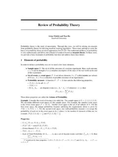
2 Why is probability theory better? de Finetti: Because if you do not reason according to probability theory , you can be made to act irrationally. probability theory is key to the study of action and communication: Decision theory combines probability theory with Utility theory . Information theory is the logarithm of probability theory . probability theory gives rise to many interesting and important philosophical questions (which we will not cover). 3. The only prerequisite: Set theory A B A B A\B. A B A B A B. For simplicity, we will work (mostly) with finite sets. The extension to countably infinite sets is not difficult. The extension to uncountably infinite sets requires Measure theory . 4. probability spaces A probability space represents our uncertainty regarding an experiment. It has two parts: 1. the sample space , which is a set of outcomes; and 2. the probability measure P , which is a real function of the subsets of . P. A. P(A) . A set of outcomes A is called an event.

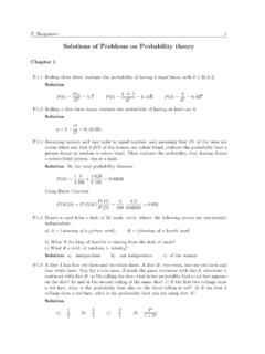
3 P (A) represents how likely it is that the experiment's actual outcome will be a member of A. 5. An example probability space If our experiment is to deploy a smoke detector and see if it works, then there could be four outcomes: = {(fire, smoke), (no fire, smoke), (fire, no smoke), (no fire, no smoke)}. Note that these outcomes are mutually exclusive. And we may choose: P ({(fire, smoke), (no fire, smoke)}) = P ({(fire, smoke), (fire, no smoke)}) = .. Our choice of P has to obey three simple rules.. 6. The three axioms of probability theory 1. P (A) 0 for all events A. 2. P ( ) = 1. 3. P (A B) = P (A) + P (B) for disjoint events A and B. B. A. 0 P(A) + P(B) = P(A B). 1. 7. Some simple consequences of the axioms P (A) = 1 P ( \A). P ( ) = 0. If A B then P (A) P (B). P (A B) = P (A) + P (B) P (A B). P (A B) P (A) + P (B).. 8. Example One easy way to define our probability measure P is to assign a probability to each outcome : fire no fire smoke no smoke These probabilities must be non-negative and they must sum to one.

4 Then the probabilities of all other events are determined by the axioms: P ({(fire, smoke), (no fire, smoke)}). = P ({(fire, smoke)}) + P ({(no fire, smoke)}). = + = 9. Conditional probability Conditional probability allows us to reason with partial information. When P (B) > 0, the conditional probability of A given B is defined as 4 P (A B). P (A | B) =. P (B). This is the probability that A occurs, given we have observed B, , that we know the experiment's actual outcome will be in B. It is the fraction of probability mass in B that also belongs to A. P (A) is called the a priori (or prior) probability of A and P (A | B) is called the a posteriori probability of A given B.. A B.. P(A B) / P(B) = P(A|B). 10. Example of conditional probability If P is defined by fire no fire smoke no smoke then P ({(fire, smoke)} | {(fire, smoke), (no fire, smoke)}). P ({(fire, smoke)} {(fire, smoke), (no fire, smoke)}). =. P ({(fire, smoke), (no fire, smoke)}). P ({(fire, smoke)}).

5 =. P ({(fire, smoke), (no fire, smoke)}). = = 11. The product rule Start with the definition of conditional probability and multiply by P (A): P (A B) = P (A)P (B | A). The probability that A and B both happen is the probability that A happens times the probability that B happens, given A has occurred. 12. The chain rule Apply the product rule repeatedly: k 1. ki=1 Ai . P = P (A1 )P (A2 | A1 )P (A3 | A1 A2 ) P Ak | i=1 Ai The chain rule will become important later when we discuss conditional independence in Bayesian networks. 13. Bayes' rule Use the product rule both ways with P (A B) and divide by P (B): P (B | A)P (A). P (A | B) =. P (B). Bayes' rule translates causal knowledge into diagnostic knowledge. For example, if A is the event that a patient has a disease, and B is the event that she displays a symptom, then P (B | A) describes a causal relationship, and P (A | B) describes a diagnostic one (that is usually hard to assess). If P (B | A), P (A) and P (B) can be assessed easily, then we get P (A | B) for free.

6 14. Random variables It is often useful to pick out aspects of the experiment's outcomes. A random variable X is a function from the sample space . X .. X( ). Random variables can define events, , { : X( ) = true}. One will often see expressions like P {X = 1, Y = 2} or P (X = 1, Y = 2). These both mean P ({ : X( ) = 1, Y ( ) = 2}). 15. Examples of random variables Let's say our experiment is to draw a card from a deck: = {A , 2 , .. , K , A , 2 , .. , K , A , 2 , .. , K , A , 2 , .. , K }. random variable example event . true if is a . H( ) = H = true false otherwise . n if is the number n N ( ) = 2<N <6. 0 otherwise . 1 if is a face card F ( ) = F =1. 0 otherwise 16. Densities Let X : be a finite random variable. The function pX : < is the density of X if for all x : pX (x) = P ({ : X( ) = x}). When is infinite, pX : < is the density of X if for all : Z. P ({ : X( ) }) = pX (x) dx . R. Note that . pX (x) dx = 1 for a valid density. X pX.. X( ) = x.

7 PX (x). 17. Joint densities If X : and Y : are two finite random variables, then pXY : < is their joint density if for all x and y : pXY (x, y) = P ({ : X( ) = x, Y ( ) = y}). When or are infinite, pXY : < is the joint density of X and Y. if for all and : Z Z. pXY (x, y) dy dx = P ({ : X( ) , Y ( ) }).. X X( ) = x pXY.. Y pXY (x,y).. Y( ) = y 18. Random variables and densities are a layer of abstraction We usually work with a set of random variables and a joint density; the probability space is implicit. pXY (x, y).. 0. 5. 5. 0. 0. y Y 5 5 x X. 19. Marginal densities Given the joint density pXY (x, y) for X : and Y : , we can compute the marginal density of X by X. pX (x) = pXY (x, y). y . when is finite, or by Z. pX (x) = pXY (x, y) dy . when is infinite. This process of summing over the unwanted variables is called marginalization. 20. Conditional densities pX|Y (x, y) : < is the conditional density of X given Y = y if pX|Y (x, y) = P ({ : X( ) = x} | { : Y ( ) = y}).

8 For all x if is finite, or if Z. pX|Y (x, y) dx = P ({ : X( ) } | { : Y ( ) = y}).. for all if is infinite. Given the joint density pXY (x, y), we can compute pX|Y as follows: pXY (x, y) pXY (x, y). pX|Y (x, y) = P 0. or pX|Y (x, y) = R 0 , y) dx0. x0 pXY (x , y) . p XY (x 21. Rules in density form Product rule: pXY (x, y) = pX (x) pY |X (y, x). Chain rule: pX1 Xk (x1 , .. , xk ). = pX1 (x1 ) pX2 |X1 (x2 , x1 ) pXk |X1 Xk 1 (xk , x1 , .. , xk 1 ). Bayes' rule: pX|Y (x, y) pY (y). pY |X (y, x) =. pX (x). 22. Inference The central problem of computational probability theory is the inference problem: Given a set of random variables X1 , .. , Xk and their joint density, compute one or more conditional densities given observations. Many problems can be formulated in these terms. Examples: In our example, the probability that there is a fire given smoke has been detected is pF |S (true, true). We can compute the expected position of a target we are tracking given some measurements we have made of it, or the variance of the position, which are the parameters of a Gaussian posterior.

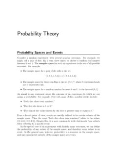
9 Inference requires manipulating densities; how will we represent them? 23. Table densities The density of a set of finite-valued random variables can be represented as a table of real numbers. In our fire alarm example, the density of S is given by . s = false pS (s) =. s = true If F is the Boolean random variable indicating a fire, then the joint density pSF is represented by pSF (s, f ) f = true f = false s = true s = false Note that the size of the table is exponential in the number of variables. 24. The Gaussian density One of the simplest densities for a real random variable. It can be represented by two real numbers: the mean and variance 2 .. P{2 < X < 3}. 0. -5 -4 -3 -2 -1 0 1 2 3 4 5. 25. The multivariate Gaussian density A generalization of the Gaussian density to d real random variables. It can be represented by a d 1 mean vector and a symmetric d d covariance matrix . 0. 5. 5. 0. 0. 5 5. 26. Importance of the Gaussian The Gaussian density is the only density for real random variables that is closed under marginalization and multiplication.

10 Also: a linear (or affine) function of a Gaussian random variable is Gaussian; and, a sum of Gaussian variables is Gaussian. For these reasons, the algorithms we will discuss will be tractable only for finite random variables or Gaussian random variables. When we encounter non-Gaussian variables or non-linear functions in practice, we will approximate them using our discrete and Gaussian tools. (This often works quite well.). 27. Looking ahead.. Inference by enumeration: compute the conditional densities using the definitions. In the tabular case, this requires summing over exponentially many table cells. In the Gaussian case, this requires inverting large matrices. For large systems of finite random variables, representing the joint density is impossible, let alone inference by enumeration. Next time: sparse representations of joint densities Variable Elimination, our first efficient inference algorithm. 28. Summary A probability space describes our uncertainty regarding an experiment; it consists of a sample space of possible outcomes, and a probability measure that quantifies how likely each outcome is.