Transcription of Simulation of Rigid Body Dynamics in Matlab
1 Simulation of Rigid body Dynamics in MatlabVarun GanapathiDepartment of PhysicsStanford UniversityMay 14, 2005 AbstractThis report presents a simulator of Rigid Dynamics of a single body in Matlab . The focus was on the conservationof Angular-Momentum and we assume that we re in the center of mass frame with no external forces. We show thatthe Simulation agrees with the analytical solution for the case of a body with two equal moments. Qualitatively, wealso show that the model exhibits the expected behavior when the moments of inertia are all different. We extend themodel to include applied torques, but the torque must be calculated analytically through some other means. We showthe numerical solution of the example of a Rigid body with two rockets on eachside of an ellipsoid, aimed to provideequal and opposite forces, and thus some total torque about the z-axisin the inertial IntroductionMany think of classical mechanics as highly intuitive and easy to visualize.
2 However, even in what is the most wellunderstood area of physics, there are still behaviors that arise that are surprising and unexpected. An example is thebehavior of a free body rotating in space. Most people would expect that a body simply rotating should generallycontinue to rotate at the same rate about the same axis in the absence of torque, while this in fact generally untrue.`and are not always in the same , it is not the case that Rigid body Dynamics rarely fact, many objects in the real world exhibit theseeffects. If the angular momentum and angular velocity vector of a car s tires don t align, the passengers will feel anuncomfortable vibration due to the precession of the tire about the angular momentum vector. In a helicopter, therotor disc has a large moment of inertia and spins quickly, therefore having a large angular momentum, which hassignificant effect on the helicopter s handling in the paper describes a way to numerically solve the equations of motion for a rotating Rigid body .
3 The Eulerequations, found in any graduate level mechanics text, formthe foundation of our method. [1] From there, we writethe first order differential equation relating orientationrepresented as quaternion to the angular velocity. The Runge-Kutta method is used to integrate the resulting coupled pairof first order differential Equations of MotionHere we summarize the physics relating to Rigid body rotation. Angular Velocity uis a vector quantity. The magni-tude of represents the rate of rotation about the axis defined by the unit vectoru. The velocity of a point on a bodyrotating with angular velocity is given byv= rwhich leads to the equation relating the derivative of a vector in an inertial reference frame to the derivative in referenceframe rotating with angular velocity :ddt(Qinertial) =ddt(Qbody) + Q(1)1 Every Rigid body has an associated inertia tensor (2) that issymmetric and real-valued, shown here with summa-tions.
4 For continuous bodies, the sums are trivially replaced with m(y2+z2) mxy mxz myx m(x2+z2) myz mzx mzy m(x2+y2) (2)The Principal Axis of a body (about an origin O) is any axis through O with the property that if points along theaxis, then`= . In other words, the principal axes are the eigenvectors of the inertia tensor. (2) It is always possibleto choose a coordinate system such that the inertia tensor isa diagonal matrix. This is a direct result of a mathematicaltheorem stating that any real symmetric matrix is momentum is now defined as the inertia tensorImultiplied in the normal matrix fashion with the angularvelocity vector .`=I (3)The law of conservation of angular momentum states thatddt`= (4)In the case of zero torque, applying (1) to`, substituting (2) and expanding the cross product results in the Eulerequations 1=( 2 3 1) 2 3 2=( 3 1 2) 3 1(5) 3=( 1 2 3) 1 2where iis theithdiagonal element of the inertia tensor.
5 It is important to remember that in the Euler equations, iistheithelement of expressed in the principal axis frame. This is why the the off-axis terms ofI(2) do not appear inthe Euler equations(5).3 Numerical Solution of EquationsThe Euler equations can be written in vector form asI =` (6)where all the quantities are expressed in the principal axisframe. Since the angular velocity equation is independent ofall other state variables in the Simulation , we can considersolving the problem in two steps. The first step is to simulatethe evolution of the angular velocity vector in the body frame, and the second step is to solve for the for Angular Velocity in the body FrameThe solution (t+dt)given (t)is straight-forward. In Matlab , based on the vector form of the Euler equations, wecan write a function giving as:function [Wdot] = getWdot( W, T, I )Imat = diag( I);Imat_inv = diag( 1 ./ I );Wdot = Imat_inv*cross( Imat*W, W );2 10010 10010 10 50510 XYZ 101 101 1 : 1: Superimposed analytical and numerical Solution for a symmetrical top with initial I = [2 2 8], W = [1 0 1] (The solutions are indistinguishable in this view)Then we can numerically integrate using fourth order Runge-Kutta:k_w(:,1) = dt*getWdot( W, t, I );k_w(:,2) = dt*getWdot( W+.)
6 5*k_w(:,1), t+.5*dt, I);k_w(:,3) = dt*getWdot( W+.5*k_w(:,2), t+.5*dt, I );k_w(:,4) = dt*getWdot( W+k_w(:,3), t + dt, I );W = W + (1/6)*( k_w*[1;2;2;1]);We can test the part of the code simulating the evolution of in the body frame for the simple case in which twoof the three terms of the diagonalized inertia tensor are equal: 1= 2< 3In this case, with the intial = [ 00 3], we can show that the analytical solution[2] of is: = [( 0cos( t)),( 0cos( t)), 3)]where = 3 1 1 3 The figure(1) shows the numerical and analytical solutions forwb(t)superimposed on the right side. In the diagramthe oval is actually a circle plotted analytically using plot3 viewed from an oblong angle. The two are completelycoincident, at least at the resolution of the figure. Figure(2) shows the plot of error as a function of time for the OrientationIn the case of linear motion, we found that we could write two coupled first order differential equations describing themotion.
7 X(t) =v(t) v(t) =f(x, v, t)3 2 1 10 5 2 1 10 5 Figure 2: Error in prediction of shown for 300 time steps. The y axis the error in y, x is error in x, both in unitsof10 5rad/s. The error spirals outward gradually with f is the force as a function of position, velocity and time. To solve that problem we interleaved the Runge-Kuttaupdates to integrate the coupled equations. Similarly, in this case, we can imagine a variableQthat represents theorientation. The derivative of the orientation is some function of .It is possible to use Euler angles to represent orientations, but there are two problems that would occur. The first isthat there is a problem known as gimbal lock where two of the rotational axes of an object merge together. After thishappens, it is essentially impossible to rotate about one ofthe three dimensions. For more details, see [3]. Second,the integration of Euler angles requires many evaluations of trigonometric functions which are generally slower are four-dimensional unit vectors of the formQ= [sv], developed by the physicist Hamilton.
8 Torepresent a rotation of angle about a given axisu, one can write the quaternionQ= [cos( 2) sin( 2) u]Many operations are defined for quaternions. The most important for the purpose of this paper is the formula convertinga quaternion into a rotation 1 2v2y 2v2z2vxvy 2svz2vxvz+ 2svy2vxvy+ 2svz1 2vxvx 2vzvz2vyvz 2svx2vxvz 2svy2vyvz+ 2svx1 2vxvx 2vyvy (7)If a quaternion represents the orientation of a Rigid body , thenrw=Rqrb, whererbis a column vector[xyz]represents a point in the frame of the Rigid body , andrwrepresents the same point in the world quaternion can also be thought of as representing a rotation. Multiplying two quaternionsp,q, gives a quaternionthat represents the application of the rotations represented bypandqin q2(8)= [s1s2 v1 v2, s1 v2+s2v1+v1 v2](9)In order to integrate the orientation, the following formula giving the derivative of the quaternion as a function oforientation and angular velocity in the world frame is also required: Q= [0w] Q4where [0 w] is interpreted as a quaternion and the rules for quaternion multiplication applied (8).
9 Due to numericalerror, a quaternion may gradually drift from having unit length. It turns out that the correct way to deal with thisproblem is to simply re-normalize the quaternion so that it points in the same direction but has unit OrientationTo find the derivative of the quaternion representation of the orientation at each time step given the angular velocity inthe body frame and the current orientation of the Rigid body ,we apply the following Find the rotation matrix representing the current orientation of the Rigid body2. Rotate binto the world frame3. Find QgivenQ, wIn Matlab , the code is:function [qdot] = getQdot(w q )R = quatToMat(q); w_inl = R*w;We can then apply fourth-order Runge-Kutta in Matlab as follows. In the code shown here,Q,Ware respectivelyquaternions representing the orientation and the angular Integrate W to find Wnew in body framek_q(:,1) = dt*getQdot( W, Q );k_w(:,1) = dt*getWdot( W, t, I );k_q(:,2) = dt*getQdot( W+.)
10 5*k_w(:,1), Q+.5*k_q(:,1) );k_w(:,2) = dt*getWdot( W+.5*k_w(:,1), t+.5*dt, I);k_q(:,3) = dt*getQdot( W+.5*k_w(:,2), Q+.5*k_q(:,2) );k_w(:,3) = dt*getWdot( W+.5*k_w(:,2), t+.5*dt, I );k_q(:,4) = dt*getQdot( W+k_w(:,3), Q+k_q(:,3) );k_w(:,4) = dt*getWdot( W+k_w(:,3), t + dt, I );Q = Q + (1/6)*( k_q*[1;2;2;1]);W = W + (1/6)*( k_w*[1;2;2;1]);% renormalize qQ = Q ./ sqrt(dot(Q,Q));4 Analytical Solution of a simple case and comparisonTo evaluate the correctness of our model , we continue considering the case of a symmetric top with two momentsof inertia equal and one moment of inertia greater. We take the derivation of the analytical solution given here fromLandau. Let us denote the principal axes with the same eigenvalue asx1, x2andx3as the principal axis with thelargest moment of inertia. Since 1== 2, we can rotatex1andx2axes aboutx3arbitrarily. In other words, becausethe top is symmetric aboutx3, any choice ofx1, x2such that they are orthogonal to each other andx3is valid.