Transcription of 2 Graphical Models in a Nutshell - ai.stanford.edu
1 2 Graphical Models in a Nutshell Daphne koller , Nir Friedman, Lise Getoor and Ben Taskar Probabilistic Graphical Models are an elegant framework which combines uncer- tainty (probabilities) and logical structure (independence constraints) to compactly represent complex, real-world phenomena. The framework is quite general in that many of the commonly proposed statistical Models (Kalman lters, hidden Markov Models , Ising Models ) can be described as Graphical Models . Graphical Models have enjoyed a surge of interest in the last two decades, due both to the exibility and power of the representation and to the increased ability to e ectively learn and perform inference in large networks. Introduction Graphical Models [11, 3, 5, 9, 7] have become an extremely popular tool for mod- eling uncertainty. They provide a principled approach to dealing with uncertainty through the use of probability theory, and an e ective approach to coping with complexity through the use of graph theory.
2 The two most common types of graph- ical Models are Bayesian networks (also called belief networks or causal networks). and Markov networks (also called Markov random elds (MRFs)). At a high level, our goal is to e ciently represent a joint distribution P over some set of random variables X = {X1 , .. , Xn }. Even in the simplest case where these variables are binary-valued, a joint distribution requires the speci cation of 2n numbers the probabilities of the 2n di erent assignments of values x1 , .. , xn . However, it is often the case that there is some structure in the distribution that allows us to factor the representation of the distribution into modular components. The structure that Graphical Models exploit is the independence properties that exist in many real-world phenomena. The independence properties in the distribution can be used to represent such high-dimensional distributions much more compactly.
3 Probabilistic Graphical mod- els provide a general-purpose modeling language for exploiting this type of structure in our representation. Inference in probabilistic Graphical Models provides us with 14 Graphical Models in a Nutshell the mechanisms for gluing all these components back together in a probabilistically coherent manner. E ective learning, both parameter estimation and model selec- tion, in probabilistic Graphical Models is enabled by the compact parameterization. This chapter provides a compact Graphical Models tutorial based on [8]. We cover representation, inference, and learning. Our tutorial is not comprehensive; for more details see [8, 11, 3, 5, 9, 4, 6]. Representation The two most common classes of Graphical Models are Bayesian networks and Markov networks. The underlying semantics of Bayesian networks are based on directed graphs and hence they are also called directed Graphical Models .
4 The underlying semantics of Markov networks are based on undirected graphs; Markov networks are also called undirected Graphical Models . It is possible, though less common, to use a mixed directed and undirected representation (see, for example, the work on chain graphs [10, 2]); however, we will not cover them here. Basic to our representation is the notion of conditional independence: De nition Let X, Y , and Z be sets of random variables. X is conditionally independent of Y given Z in a distribution P if P (X = x, Y = y | Z = z) = P (X = x | Z = z)P (Y = y | Z = z). for all values x V al(X), y V al(Y ) and z V al(Z). In the case where P is understood, we use the notation (X Y | Z) to say that X. is conditionally independent of Y given Z. If it is clear from the context, sometimes we say independent when we really mean conditionally independent.
5 Bayesian Networks The core of the Bayesian network representation is a directed acyclic graph (DAG). G. The nodes of G are the random variables in our domain and the edges correspond, intuitively, to direct in uence of one node on another. One way to view this graph is as a data structure that provides the skeleton for representing the joint distribution compactly in a factorized way. Let G be a BN graph over the variables X1 , .. , Xn . Each random variable Xi in the network has an associated conditional probability distribution (CPD) or local probabilistic model. The CPD for Xi , given its parents in the graph (denoted PaXi ), is P (Xi | PaXi ). It captures the conditional probability of the random variable, given its parents in the graph. CPDs can be described in a variety of ways. A. common, but not necessarily compact, representation for a CPD is a table which contains a row for each possible set of values for the parents of the node describing Representation 15.
6 P(P) P(T). P T P(I |P, T ). p t p t P T. Pneumonia Tuberculosis p t p t I S P(S|T ). Lung Infiltrates I P(X|I ) s i s XRay Sputum Smear i X S. (a) (b). Figure (a) A simple Bayesian network showing two potential diseases, Pneu- monia and Tuberculosis, either of which may cause a patient to have Lung Infiltrates. The lung in ltrates may show up on an XRay ; there is also a separate Sputum Smear test for tuberculosis. All of the random variables are Boolean. (b) The same Bayesian network, together with the conditional probability tables. The probabili- ties shown are the probability that the random variable takes the value true (given the values of its parents); the conditional probability that the random variable is false is simply 1 minus the probability that it is true. the probability of di erent values for Xi . These are often referred to as table CPD s, and are tables of multinomial distributions.
7 Other possibilities are to represent the distributions via a tree structure (called, appropriately enough, tree-structured CPDs), or using an even more compact representation such as a noisy-OR or noisy- MAX. Example Consider the simple Bayesian network shown in gure This is a toy example indicating the interactions between two potential diseases, pneumonia and tuber- culosis. Both of them may cause a patient to have lung in ltrates. There are two tests that can be performed. An x-ray can be taken, which may indicate whether the patient has lung in ltrates. There is a separate sputum smear test for tubercu- losis. gure (a) shows the dependency structure among the variables. All of the variables are assumed to be Boolean. gure (b) shows the conditional probability distributions for each of the random variables. We use initials P , T , I, X, and S.
8 For shorthand. At the roots, we have the prior probability of the patient having each disease. The probability that the patient does not have the disease a priori is simply 1 minus the probability he or she has the disease; for simplicity only the probabilities for the true case are shown. Similarly, the conditional probabilities for the non-root nodes give the probability that the random variable is true, for di erent possible instantiations of the parents. 16 Graphical Models in a Nutshell De nition Let G be a Bayesinan network graph over the variables X1 , .. , Xn . We say that a distribution PB over the same space factorizes according to G if PB can be expressed as a product . n PB (X1 , .. , Xn ) = P (Xi | PaXi ). ( ). i=1. A Bayesian network is a pair (G, G ) where PB factorizes over G, and where PB is speci ed as set of CPDs associated with G's nodes, denoted G.
9 The equation above is called the chain rule for Bayesian networks. It gives us a method for determining the probability of any complete assignment to the set of random variables: any entry in the joint can be computed as a product of factors, one for each variable. Each factor represents a conditional probability of the variable given its parents in the network. Example The Bayesian network in gure (a) describes the following factorization: P (P, T, I, X, S) = P (P )P (T )P (I | P, T )P (X | I)P (S | T ). Sometimes it is useful to think of the Bayesian network as describing a generative process. We can view the graph as encoding a generative sampling process executed by nature, where the value for each variable is selected by nature using a distribution that depends only on its parents. In other words, each variable is a stochastic function of its parents.
10 Conditional Independence Assumptions in Bayesian Networks Another way to view a Bayesian network is as a compact representation for a set of conditional independence assumptions about a distribution. These conditional independence assumptions are called the local Markov assumptions. While we won't go into the full details here, this view is, in a strong sense, equivalent to the view of the Bayesian network as providing a factorization of the distribution. De nition Given a BN network structure G over random variables X1 , .. , Xn , let NonDescendantsXi denote the variables in the graph that are not descendants of Xi . Then G encodes the following set of conditional independence assumptions, called the local Markov assumptions: For each variable Xi , we have that (Xi NonDescendantsXi | PaXi ), In other words, the local Markov assumptions state that each node Xi is inde- pendent of its nondescendants given its parents.