6.1: Using the Standardized Normal Distribution …

1 : Using the Standardized Normal Distribution table CD6-1. : Using THE Standardized Normal Distribution table . Any set of normally distributed data can be converted to its Standardized form and the desired prob- abilities can then be determined from a table of the Standardized Normal Distribution . To see how the transformation Equation ( ) on page 199 can be applied and how you can use the results to obtain probabilities from the table of the Standardized Normal Distribution ( table ), consider the following problem. Suppose a consultant was investigating the time it took factory workers in an automobile plant to assemble a particular part after the workers had been trained to perform the task Using an indi- vidual learning approach. The consultant determined that the time in seconds to assemble the part for workers trained with this method was normally distributed with a mean of 75 seconds and a standard deviation of 6 seconds.

2 Transforming the Data From Figure observe that every measurement X has a corresponding Standardized measure- ment Z obtained from the transformation formula ( ). Hence from Figure a time of 81 sec- onds required for a factory worker to complete the task is equivalent to 1 Standardized unit (that is, 1 standard deviation) above the mean, since 81 75. Z = = +1. 6. and a time of 57 seconds required for a worker to assemble the part is equivalent to 3 Standardized units (that is, 3 standard deviations) below the mean because 57 75. Z = = 3. 6. Thus, the standard deviation has become the unit of measurement. In other words, a time of 81 sec- onds is 6 seconds ( , 1 standard deviation) higher, or slower than the average time of 75 seconds and a time of 57 seconds is 18 seconds ( , 3 standard deviations) lower, or faster than the average time.

3 Automobile Plant with Individual-Based Training 3 2 1 + 1 + 2 + 3 X Scale 57 63 69 75 81 87 93 ( = 75, = 6). FIGURE 3 2 1 0 +1 +2 +3 Z Scale Transformation of scales Suppose now that the consultant conducted the same study at another automobile plant, where the workers were trained to assemble the part by Using a team-based learning method. Suppose that at this plant the consultant determined that the time to perform the task was normally distributed with mean of 60 seconds and a standard deviation of 3 seconds. The data are depicted in Figure In comparison with the results for workers who had an individual learning method, note, for example, that at the plant where workers had team-based training, a time of 57 seconds to complete the task is only 1 standard deviation below the mean for the group, since 57 60. Z = = 1. 3. CD6-2 CD MATERIAL.

4 Note that a time of 63 seconds is 1 standard deviation above the mean time for assemblage, since 63 60. Z = = +1. 3. and a time of 51 seconds is 3 standard deviations below the group mean because 51 60. Z = = 3. 3. Using the Normal Probability Tables The two bell-shaped curves in Figures and depict the relative frequency polygons for the Normal distributions representing the time (in seconds) for all factory workers to assemble a part at two automobile plants, one that employed individual-based training and the other that employed team-based training. Since at each plant the times to assemble the part are known for every factory worker, the data represent the entire population at a particular plant, and therefore the probabilities or proportion of area under the entire curve must add up to 1. Thus, the area under the curve between any two reported times values represents only a portion of the total area possible.

5 Automobile Plant with Team-Based Training 51 54 57 60 63 66 69 X. FIGURE A different transformation of 3 2 1 0 +1 +2 +3 Z. scales Suppose the consultant wishes to determine the probability that a factory worker selected at random from those who underwent individual-based training should require between 75 and 81. seconds to complete the task. That is, what is the likelihood that the worker's time is between the plant mean and one standard deviation above this mean? This answer is found by Using table table represents the probabilities or areas under the Normal curve calculated from the mean to the particular values of interest X. Using Equation ( ), this corresponds to the probabil- ities or areas under the Standardized Normal curve from the mean to the transformed values of interest Z. Only positive entries for Z are listed in the table , since for a symmetrical Distribution hav- ing a mean of zero, the area from the mean to +Z (that is, Z standard deviations above the mean).

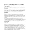
6 Must be identical to the area from the mean to Z (that is, Z standard deviations below the mean). : Using the Standardized Normal Distribution table CD6-3. To use table note that all Z values must first be recorded to two decimal places. Thus the Z. value of interest is recorded as + To read the probability or area under the curve from the mean to Z = + , scan down the Z column from table until you locate the Z value of interest (in tenths). Hence you stop in the row Z = Next read across this row until you intersect the column that contains the hundredths place of the Z value. Therefore, in the body of the table the tabulated probability for Z = corresponds to the intersection of the row Z = with the column Z = .00. as shown in table (which is a portion of table ). This probability is As depicted in Figure , there is a chance that a factory worker selected at random who has had individ- ual-based training will require between 75 and 81 seconds to assemble the part.

7 table Z .00 .01 .02 .03 .04 .05 .06 .07 .08 .09. Obtaining an area under the Normal curve .0000 .0040 .0080 .0120 .0160 .0199 .0239 .0279 .0319 .0359..0398 .0438 .0478 .0517 .0557 .0596 .0636 .0675 .0714 .0753..0793 .0832 .0871 .0910 .0948 .0987 .1026 .1064 .1103 .1141..1179 .1217 .1255 .1293 .1331 .1368 .1406 .1443 .1480 .1517..1554 .1591 .1628 .1664 .1700 .1736 .1772 .1808 .1844 .1879..1915 .1950 .1985 .2019 .2054 .2088 .2123 .2157 .2190 .2224..2257 .2291 .2324 .2357 .2389 .2422 .2454 .2486 .2518 .2549..2580 .2612 .2642 .2673 .2704 .2734 .2764 .2794 .2823 .2852..2881 .2910 .2939 .2967 .2995 .3023 .3051 .3078 .3106 .3133..3159 .3186 .3212 .3238 .3264 .3289 .3315 .3340 .3365 .3389..3413 .3438 .3461 .3485 .3508 .3531 .3554 .3577 .3599 .3621..3643 .3665 .3686 .3708 .3729 .3749 .3770 .3790 .3810 .3830. Source: Extracted from table Automobile Plant X 81 75.

8 Z= = = + with Individual-Based 2. Training Area .3413. FIGURE 57 63 69 75 81 87 93 X Scale Determining the area between the mean and Z from a 0 + + + Z Scale Standardized Normal Distribution On the other hand, you know from Figure that at the automobile plant where the workers received team-based training, a time of 63 seconds is 1 Standardized unit above the mean time of 60. seconds. Thus the likelihood that a randomly selected factory worker who received team-based training will complete the assemblage in between 60 and 63 seconds is also These results are illustrated in Figure , which demonstrates that regardless of the value of the mean and stan- dard deviation of a particular set of normally distributed data, a transformation to a Standardized scale can always be made from Equation ( ), and, by Using table , any probability or portion of area under the curve can be obtained.

9 From Figure you see that the probability or area under the curve from 60 to 63 seconds for the workers who had team-based training is identical to the probability or area under the curve from 75 to 81 seconds for the workers who had individual-based training. CD6-4 CD MATERIAL. Team-Based Training e Individual-Based Training cal XS. 93. 87. 81. 75 e 69 cal 63 ZS. 57. 51 +3. +2. +1. 0. 1. FIGURE 2. Demonstrating a transformation of scales for corresponding 3. portions under two Normal curves Now that you have learned to use table in conjunction with Equation ( ), many different types of probability questions pertaining to the Normal Distribution can be resolved. To illustrate, suppose that the consultant raises the following questions with regard to assembling a particular part by workers who had individual-based training: 1. What is the probability that a randomly selected factory worker can assemble the part in under 75 seconds or in over 81 seconds?

10 2. What is the probability that a randomly selected factory worker can assemble the part in 69. to 81 seconds? 3. What is the probability that a randomly selected factory worker can assemble the part in under 62 seconds? 4. What is the probability that a randomly selected factory worker can assemble the part in 62. to 69 seconds? 5. How many seconds must elapse before 50% of the factory workers assemble the part? 6. How many seconds must elapse before 10% of the factory workers assemble the part? 7. What is the interquartile range (in seconds) expected for factory workers to assemble the part? Finding the Probabilities Corresponding to Known Values Recall that for workers who had individual-based training the assembly time data are normally dis- tributed with a mean of 75 seconds and a standard deviation of 6 seconds. In responding to questions 1 through 4, this information is used to determine the probabilities associated with vari- ous measured values.