6 Probability Density Functions (PDFs)

1 CSC 411 / CSC D11 / CSC C11 Probability Density Functions (PDFs) 6 probability density functions (PDFs)In many cases, we wish to handle data that can be represented as a real-valued random variable,or a real-valued vectorx= [x1, x2, .., xn]T. Most of the intuitions from discrete variables transferdirectly to the continuous case, although there are some describe the probabilities of a real-valued scalar variablexwith a Probability DensityFunction (PDF), writtenp(x). Any real-valued functionp(x)that satisfies:p(x) 0for allx(1) p(x)dx= 1(2)is a valid PDF. I will use the convention of upper-casePfor discrete probabilities, and lower-casepfor the PDF we can specify the Probability that the random variablexfalls within a givenrange:P(x0 x x1) = x1x0p(x)dx(3)This can be visualized by plotting the curvep(x).

2 Then, to determine the Probability thatxfallswithin a range, we compute the area under the curve for that PDF can be thought of as the infinite limit of a discrete distribution, , a discrete dis-tribution with an infinite number of possible outcomes. Specifically, suppose we create a discretedistribution withNpossible outcomes, each corresponding to a range on the realnumber , suppose we increaseNtowards infinity, so that each outcome shrinks to a single real num-ber; a PDF is defined as the limiting case of this discrete is an important subtlety here: a Probability Density isnota Probability per se. Forone thing, there is no requirement thatp(x) 1. Moreover, the Probability thatxattains anyone specific value out of the infinite set of possible values isalways zero, (x= 5) = 55p(x)dx= 0for any PDFp(x).

3 People (myself included) are sometimes sloppy in referringtop(x)as a Probability , but it is not a Probability rather, it is a function that can be used incomputing distributions are defined in a natural way. For two variablesxandy, the joint PDFp(x, y)defines the Probability that(x, y)lies in a given domainD:P((x, y) D) = (x,y) Dp(x, y)dxdy(4)For example, the Probability that a 2D coordinate(x, y)lies in the domain(0 x 1,0 y 1)is 0 x 1 0 y 1p(x, y)dxdy. The PDF over a vector may also be written as a joint PDF of itsvariables. For example, for a 2D-vectora= [x, y]T, the PDFp(a)is equivalent to the PDFp(x, y).Conditional distributions are defined as well:p(x|A)is the PDF overx, if the statementAistrue. This statement may be an expression on a continuous value, y= 5.

4 As a short-hand,Copyrightc 2015 Aaron Hertzmann, David J. Fleet and Marcus Brubaker27 CSC 411 / CSC D11 / CSC C11 Probability Density Functions (PDFs)we can writep(x|y), which provides a PDF forxfor every value ofy. (It must be the case that p(x|y)dx= 1, sincep(x|y)is a PDF over values ofx.)In general, for all of the rules for manipulating discrete distributions there are analogous rulesfor continuous distributions: Probability rules for PDFs: p(x) 0, for allx p(x)dx= 1 P(x0 x x1) = x1x0p(x)dx Sum rule: p(x)dx= 1 Product rule:p(x, y) =p(x|y)p(y) =p(y|x)p(x). Marginalization:p(y) = p(x, y)dx We can also add conditional information, (y|z) = p(x, y|z)dx Independence:Variablesxandyare independent if:p(x, y) =p(x)p(y). Mathematical expectation, mean, and varianceSome very brief definitions of ways to describe a PDF:Given a functionf(x)of an unknown variablex, theexpected valueof the function with repectto a PDFp(x)is defined as:Ep(x)[f(x)] f(x)p(x)dx(5)Intuitively, this is the value that we roughly expect xto mean of a distributionp(x)is the expected value ofx: =Ep(x)[x] = xp(x)dx(6)The variance of a scalar variablexis the expected squared deviation from the mean:Ep(x)[(x )2] = (x )2p(x)dx(7)The variance of a distribution tells us how uncertain, or spread-out the distribution is.

5 For a verynarrow distributionEp(x)[(x )2]will be a vectorxis a matrix: = cov(x) =Ep(x)[(x )(x )T] = (x )(x )Tp(x)dx(8)By inspection, we can see that the diagonal entries of the covariance matrix are the variances ofthe individual entries of the vector: ii= var(xii) =Ep(x)[(xi i)2](9)Copyrightc 2015 Aaron Hertzmann, David J. Fleet and Marcus Brubaker28 CSC 411 / CSC D11 / CSC C11 Probability Density Functions (PDFs)The off-diagonal terms are covariances: ij= cov(xi, xj) =Ep(x)[(xi i)(xj j)](10)between variablesxiandxj. If the covariance is a large positive number, then we expectxito belarger than iwhenxjis larger than j. If the covariance is zero and we know no other information,then knowingxi> idoes not tell us whether or not it is likely thatxj> goal of statistics is to infer properties of distributions.

6 In the simplest case, thesamplemeanof a collection ofNdata pointsx1:Nis just their average: x=1N ixi. Thesamplecovarianceof a set of data points is:1N i(xi x)(xi x)T. The covariance of the data pointstells us how spread-out the data points Uniform distributionsThe simplest PDF is theuniform distribution. Intuitively, this distribution states that all valueswithin a given range[x0, x1]are equally likely. Formally, the uniform distribution on the interval[x0, x1]is:p(x) ={1x1 x0ifx0 x x10otherwise(11)It is easy to see that this is a valid PDF (becausep(x)>0and p(x)dx= 1).We can also write this distribution with this alternative notation:x|x0, x1 U(x0, x1)(12)Equations 11 and 12 are equivalent. The latter simply says:xis distributed uniformly in the rangex0andx1, and it is impossible thatxlies outside of that mean of a uniform distributionU(x0, x1)is(x1+x0)/2.}

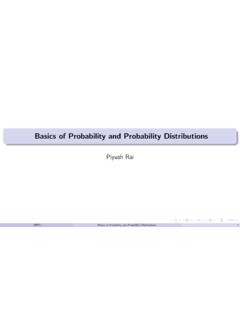
7 The variance is(x1 x0)2 Gaussian distributionsArguably the single most important PDF is theNormal( ,Gaussian) Probability distributionfunction (PDF). Among the reasons for its popularity are that it is theoretically elegant, and arisesnaturally in a number of situations. It is the distribution that maximizes entropy, and it is also tiedto the Central Limit Theorem: the distribution of a random variable which is the sum of a numberof random variables approaches the Gaussian distribution as that number tends to infinity (Figure1).Perhaps most importantly, it is the analytical properties of the Gaussian that make it so ubiqui-tous. Gaussians are easy to manipulate, and their form so well understood, that we often assumequantities are Gaussian distributed, even though they are not, in order to turn an intractable model,or problem, into something that is easier to work 2015 Aaron Hertzmann, David J.

8 Fleet and Marcus Brubaker29 CSC 411 / CSC D11 / CSC C11 Probability Density Functions (PDFs)N= 1: Histogram plots of the mean ofNuniformly distributed numbers for various values ofN. The effect of the Central Limit Theorem is seen: asNincreases, the distribution becomes moreGaussian.(Figure fromPattern Recognition and Machine Learningby Chris Bishop.)The simplest case is a Gaussian PDF over a scalar valuex, in which case the PDF is:p(x| , 2) =1 2 2exp( 12 2(x )2)(13)(The notationexp(a)is the same asea). The Gaussian has two parameters, the mean , andthe variance 2. The mean specifies the center of the distribution, and the variance tells us how spread-out the PDF PDF forD-dimensional vectorx, the elements of which are jointly distributed with a theGaussian denity function, is given byp(x| , ) =1 (2 )D| |exp( (x )T 1(x )/2)(14)where is the mean vector, and is theD Dcovariance matrix, and|A|denotes the determinantof matrixA.

9 An important special case is when the Gaussian is isotropic(rotationally invariant).In this case the covariance matrix can be written as = 2 IwhereIis the identity matrix. This iscalled a spherical or isotropic covariance matrix. In this case, the PDF reduces to:p(x| , 2) =1 (2 )D 2 Dexp( 12 2||x ||2).(15)The Gaussian distribution is used frequently enough that itis useful to denote its PDF in asimple way. We will define a functionGto be the Gaussian Density function, ,G(x; , ) 1 (2 )D| |exp( (x )T 1(x )/2)(16)When formulating problems and manipulating PDFs this functional notation will be useful. Whenwe want to specify that a random vector has a Gaussian PDF, it is common to use the notation:x| , N( , )(17)Copyrightc 2015 Aaron Hertzmann, David J.

10 Fleet and Marcus Brubaker30 CSC 411 / CSC D11 / CSC C11 Probability Density Functions (PDFs)Equations 14 and 17 essentially say the same thing. Equation17 says thatxis Gaussian, andEquation 14 specifies (evaluates) the Density for an inputx. The covariance matrix of a Gaussianmust be symmetric and positive DiagonalizationA useful way to understand a Gaussian is to diagonalize the exponent. The exponent of the Gaus-sian is quadratic, and so its shape is essentially elliptical. Through diagonalization we find themajor axes of the ellipse, and the variance of the distribution along those axes. Seeing the Gaus-sian this way often makes it easier to interpret the a reminder, the eigendecomposition of a real-valued symmetric matrix yields a set oforthonormal vectorsviand scalars isuch that ui= iui(18)Equivalently, if we combine the eigenvalues and eigenvectors into matricesU= [u1.]