Basics of Probability and Probability Distributions

1 Basics of Probability and Probability Distributions Piyush Rai (IITK) Basics of Probability and Probability Distributions 1. Some Basic Concepts You Should Know About Random variables (discrete and continuous). Probability Distributions over discrete/continuous 's Notions of joint, marginal, and conditional Probability Distributions Properties of random variables (and of functions of random variables). Expectation and variance/covariance of random variables Examples of Probability Distributions and their properties Multivariate Gaussian distribution and its properties (very important). Note: These slides provide only a (very!) quick review of these things. Please refer to a text such as PRML (Bishop) Chapter 2 + Appendix B, or MLAPP (Murphy) Chapter 2 for more details Note: Some other pre-requisites ( , concepts from information theory, linear algebra, optimization, etc.)

2 Will be introduced as and when they are required (IITK) Basics of Probability and Probability Distributions 2. Random Variables Informally, a random variable ( ) X denotes possible outcomes of an event Can be discrete ( , finite many possible outcomes) or continuous Some examples of discrete A random variable X {0, 1} denoting outcomes of a coin-toss A random variable X {1, 2, .. , 6} denoteing outcome of a dice roll Some examples of continuous A random variable X (0, 1) denoting the bias of a coin A random variable X denoting heights of students in this class A random variable X denoting time to get to your hall from the department (IITK) Basics of Probability and Probability Distributions 3. Discrete Random Variables For a discrete X , p(x) denotes the Probability that p(X = x).

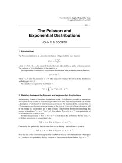
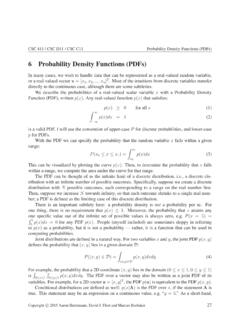
3 P(x) is called the Probability mass function (PMF). p(x) 0. p(x) 1. X. p(x) = 1. x (IITK) Basics of Probability and Probability Distributions 4. Continuous Random Variables For a continuous X , a Probability p(X = x) is meaningless Instead we use p(X = x) or p(x) to denote the Probability density at X = x For a continuous X , we can only talk about Probability within an interval X (x, x + x). p(x) x is the Probability that X (x, x + x) as x 0. The Probability density p(x) satisfies the following Z. p(x) 0 and p(x)dx = 1 (note: for continuous , p(x) can be > 1). x (IITK) Basics of Probability and Probability Distributions 5. A word about p(.) can mean different things depending on the context p(X ) denotes the distribution (PMF/PDF) of an X.

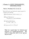
4 P(X = x) or p(x) denotes the Probability or Probability density at point x Actual meaning should be clear from the context (but be careful). Exercise the same care when p(.) is a specific distribution (Bernoulli, Beta, Gaussian, etc.). The following means drawing a random sample from the distribution p(X ). x p(X ). (IITK) Basics of Probability and Probability Distributions 6. Joint Probability distribution Joint Probability distribution p(X , Y ) models Probability of co-occurrence of two X , Y. For discrete , the joint PMF p(X , Y ) is like a table (that sums to 1). XX. p(X = x, Y = y ) = 1. x y For continuous , we have joint PDF p(X , Y ). Z Z. p(X = x, Y = y )dxdy = 1. x y (IITK) Basics of Probability and Probability Distributions 7.

5 Marginal Probability distribution Intuitively, the Probability distribution of one regardless of the value the other takes P P. For discrete 's: p(X ) = y p(X , Y = y ), p(Y ) = x p(X = x, Y ). For discrete it is the sum of the PMF table along the rows/columns R R. For continuous : p(X ) = y p(X , Y = y )dy , p(Y ) = x p(X = x, Y )dx Note: Marginalization is also called integrating out . (IITK) Basics of Probability and Probability Distributions 8. Conditional Probability distribution - Probability distribution of one given the value of the other - Conditional Probability p(X |Y = y ) or p(Y |X = x): like taking a slice of p(X , Y ). - For a discrete distribution : - For a continuous distribution1 : 1 Picture courtesy: Computer vision: models, learning and inference (Simon Price).

6 (IITK) Basics of Probability and Probability Distributions 9. Some Basic Rules Sum rule: Gives the marginal Probability distribution from joint Probability distribution P. For discrete : p(X ) = Y p(X , Y ). R. For continuous : p(X ) = Y. p(X , Y )dY. Product rule: p(X , Y ) = p(Y |X )p(X ) = p(X |Y )p(Y ). Bayes rule: Gives conditional Probability p(X |Y )p(Y ). p(Y |X ) =. p(X ). For discrete : p(Y |X ) = Pp(X |Y )p(Y ). Y p(X |Y )p(Y ). For continuous : p(Y |X ) = R p(X |Y )p(Y ). Y p(X |Y )p(Y )dY. Also remember the chain rule p(X1 , X2 , .. , XN ) = p(X1 )p(X2 |X1 ) .. p(XN |X1 , .. , XN 1 ). (IITK) Basics of Probability and Probability Distributions 10. Independence X and Y are independent (X . Y ) when knowing one tells nothing about the other p(X |Y = y ) = p(X ).

7 P(Y |X = x) = p(Y ). p(X , Y ) = p(X )p(Y ). X . Y is also called marginal independence Conditional independence (X . Y |Z ): independence given the value of another Z. p(X , Y |Z = z) = p(X |Z = z)p(Y |Z = z). (IITK) Basics of Probability and Probability Distributions 11. Expectation Expectation or mean of an with PMF/PDF p(X ). X. E[X ] = xp(x) (for discrete Distributions ). x Z. E[X ] = xp(x)dx (for continuous Distributions ). x Note: The definition applies to functions of too ( , E[f (X )]). Linearity of expectation E[ f (X ) + g (Y )] = E[f (X )] + E[g (Y )]. (a very useful property, true even if X and Y are not independent). Note: Expectations are always the underlying Probability distribution of the random variable involved, so sometimes we'll write this explicitly as Ep() [.]

8 ], unless it is clear from the context (IITK) Basics of Probability and Probability Distributions 12. Variance and Covariance Variance 2 (or spread around mean ) of an with PMF/PDF p(X ). var[X ] = E[(X )2 ] = E[X 2 ] 2. p Standard deviation: std[X ] = var[X ] = . For two scalar 's x and y , the covariance is defined by cov[x, y ] = E [{x E[x]}{y E[y ]}] = E[xy ] E[x]E[y ]. For vector x and y , the covariance matrix is defined as cov[x, y ] = E {x E[x]}{y T E[y T ]} = E[xy T ] E[x]E[y > ].. Cov. of components of a vector x: cov[x] = cov[x, x]. Note: The definitions apply to functions of too ( , var[f (X )]). Note: Variance of sum of independent 's: var[X + Y ] = var[X ] + var[Y ]. (IITK) Basics of Probability and Probability Distributions 13.

9 Transformation of Random Variables Suppose y = f (x) = Ax + b be a linear function of an x Suppose E[x] = and cov[x] = . Expectation of y E[y ] = E[Ax + b] = A + b Covariance of y cov[y ] = cov[Ax + b] = A AT. Likewise if y = f (x) = a T x + b is a scalar-valued linear function of an x: E[y ] = E[a T x + b] = a T + b var[y ] = var[a T x + b] = a T a Another very useful property worth remembering (IITK) Basics of Probability and Probability Distributions 14. Common Probability Distributions Important: We will use these extensively to model data as well as parameters Some discrete Distributions and what they can model: Bernoulli: Binary numbers, , outcome (head/tail, 0/1) of a coin toss Binomial: Bounded non-negative integers, , # of heads in n coin tosses Multinomial: One of K (>2) possibilities, , outcome of a dice roll Poisson: Non-negative integers, , # of words in a document.

10 And many others Some continuous Distributions and what they can model: Uniform: numbers defined over a fixed range Beta: numbers between 0 and 1, , Probability of head for a biased coin Gamma: Positive unbounded real numbers Dirichlet: vectors that sum of 1 (fraction of data points in different clusters). Gaussian: real-valued numbers or real-valued vectors .. and many others (IITK) Basics of Probability and Probability Distributions 15. Discrete Distributions (IITK) Basics of Probability and Probability Distributions 16. Bernoulli distribution distribution over a binary x {0, 1}, like a coin-toss outcome Defined by a Probability parameter p (0, 1). P(x = 1) = p distribution defined as: Bernoulli(x; p) = p x (1 p)1 x Mean: E[x] = p Variance: var[x] = p(1 p).