7 Wing Design - HAW Hamburg

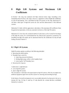
1 7 - 17 Wing DesignDuring the preliminary sizing, the wing was merely described in terms of the wing area SW and the wing aspect ratioAW. When designing the wing, other wing parameters are determ ined. This involves the definition of the wing section and the Wing ParametersFig. of the wing sectionsWing sections are positioned parallel to the plane of symmetry of the aircraft (Fig. ). A wing section is produced by scaling up an airfoil section . The airfoil section is described by the section coordinates of the top of the section yf xu=( ) and the bottom of the section yf xl=( ) with01 x. Sections can also be described by the thickness distribution tf x=( ) combined with the camberyf xc=( ). Fig. contains additional parameters for describing the section geometry:Chord c Thickness tCamber ( ) /yccmaxPosition of maximum thickness xtPosition of maximum camberxycmax( )Leading edge radius rTrailing edge angle TE7 - 2 Fig. also defines the following:Chord line(Mean) camber lineLeading edgeLETrailing edgeTEFig.

2 :Airfoil geometry (DATCOM 1978)For simplicity of production, planforms with a curved leading and trailing edge are rare. Wings can therefore very often be described as double tapered wings (Fig. ). The simple tapered wing and the rectangular wing can be seen as special versions of the double tapered wing. The sweep angle depends on the % line1 on which it is measured. Normally the sweep angle of the leading edge LE, trailing edge TE, 25% line 25 (quarter chord sweep) and 50% line 50 are point where the inner and outer taper meet is called the kink. At this kink, the local chord is called ck. In contrast to the chord at the wing tip ct a chord does not actually exist on the wing root cr, but is only created by graphically extending the leading and trailing edge as far as the plane of symmetry and therefore into the fuselage. The mean aerodynamic chord cMAC is the chord of an equivalent untwisted, unswept rectangular wing that achieves the same lift and the same pitching moment as this wing.

3 The aerodynamic center, AC lies on the mean aerodynamic chord. The aerodynamic center is characterized by the following feature: if 1n% point: point on a local chord that is located n% of the local chord behind the leading line: line formed by the geometric locations of the n% points of the : In this case n% is replaced by a percentage ( 25%) or another figure symbolizing the per centage ( c/4). 7 - 3we take an axis that is perpendicular to the plane of symmetry of the aircraft and passes through the aerodynamic center, the pitching moment of the wing about this axis is constant and independent of the lift. The position of the aerodynamic center XAC on a rectangular wing with a thin symmetrical section is 0 25. cMAC. Torenbeek 1988 (Fig. E10) contains details of the position of the aerodynamic center on simple tapered wings. Fig. of the double tapered wingWing area SW does not just include the visible part of the wing. The wing area also includes the area of the inner taper in the fuselage.

4 The exact size of the wing area is not really import ant. All that is needed for the calculations is a standard reference wing area Sref. Why is this? Let s take a look at the calculation for lift in cruise flight, for example: mgLvCSLref == 1 22/ . If Sref is changed, only the lift coefficient CL changes (by defini tion). For this reason, aircraft manufacturers often use their own in-house definition of the (reference) wing area. Fig. and Fig. show such differing definitions of the wing - 4 Fig. )Definition of the refer ence wing area accord ing to : The Boeing B-747 has a different definition of the reference wing area: Sref = )Definition of the refer ence wing area accord ing to Focker and Mc Donnell ''''2211 + +=TrapezeWingBasic:refS7 - 5 Fig. of the reference wing area according to AirbusWing parameters in aircraft designThe following have already been determined (to a large extent) (see section 5): Wing area SW Wing aspect searching for a suitable aircraft configuration (see section 4) consideration was already given to transmitting the forces from the wing to the fuselage by means of the following con figuration: cantilever wing braced wingand to the position of the wing in relation to the fuselage low wing position mid wing position high wing position7 - 6 Fig.

5 (Positive) dihedral angle of the wingW Fig. (Positive) incidence angle iW: angle between the chord line of the wing root and a reference line of the fuselage ( cabin floor) The following still have to be determined (here in section 7):Taper ratio, WSweep angle, 25 ,WThickness ratio, ()tcW/Airfoils Dihedral angle, vW (Fig. )Incidence angle, iW (Fig. )Wing twist, t (Fig. )Subsections and below contain equations and estimates for these parameters. It is im portant to compare and check the calculation results with the values from the aircraft statistics. Tables with wing parameters are, for example, included in Roskam II ( section 6) and Toren beek 1988 ( section 7). Further comprehensive information can be found in Jane's All The World's Aircraft (Lambert 1993).7 - 7 Fig. twist t. The twist shown in the diagram is negative. There are two types of wing twist: 1.)Geometric twist:change in the angle between the chord ) Aerodynamic twist:change in the zero-lift line along the span of an diagram shows the typical case of reduced lift at the wing tip, wash out.

6 The opposite effect is called wash in .The following must be taken into account when choosing parameters: Take-off/landing: maximum lift coefficient, required high lift systems, lift-to-drag ratio, at titude, lift curve slope dCdL/ Cruise: lift-to-drag ratio L/D, drag divergence Mach number MDD, buffet onset boundary Fuel tank volume Flight characteristics, stalling behavior, flight in turbulence Landing gear actuation and stowage Wing mass Production costsThese characteristics, which depend on the choice of the above-mentioned wing parameters, are discussed in Subsection DefinitionsAspect ratioAbS=2 ,( )with Span aerodynamic chordcSc dyMACb= 2202/ ,( )7 - 8 AreaSc dyb= 202/ ,( )Spanwise location of mean aerodynamic chordyScy dyMACb= 202/ .( )with y spanwise span position2/by= ,( )Taper ratio =cctr ,( )The following additionally applies to double tapered wings:on the inner wing (index: i) ikrcc= ,( )on the outer wing (index: o) otkcc= .( )Equations for the geometry of the simple tapered wingAbSbcr==+221() ,( )ccMACr=+++23112 ,( )()Sbcr=+21 ,( )ybccMACMACr/ 211131 21= =++ ,( )7 - 9 Conversion of the sweep of an m% line to the sweep of an n% line (m and n are the % values):tantan nmAnm= + 410011.

7 ( )Equations for the geometry of the double tapered wing[]AbSbcrki== ++221() ,( )with 2/bykk= .ccScSSMACMACiiMACoo= + ,, ,( )()[]SSSbAbciorki=+== ++221 ,( )()yySyySSSMACMCAiikMACooio= ++ +,, .( )Please note: The index( )W for wing was omitted in equations to because the equa tions are thus also applicable to a horizontal tailplane. When calculating the geometry of a vertical tailplane, it is important to take into account that the tailplane only consists of half the area. Thus, for example, equation ( ) can be used to produce the definition for the area of the vertical tailplane SV: Sc dyVb= 02/ .( ) Principle and Design EquationsPressure coefficientThe flow configurations around an airfoil are shown with the aid of the pressure coefficient (see Fig. ). The pressure coefficient is defined as7 - 10cppqp= ..( )The index refers to a parameter of the free flow (undisturbed by the airfoil section ). By definition: 221 =Vq and for incompressible flow (Bernoulli) 222121 VpVp +=+ hence ()2221 VVpp =.

8 With the local super velocity v= V-V () = =VvVVVVVcp2121212222 .( )The approximation ( ) applies for v much smaller than V . The local velocity at the airfoil is VVcp= 1 .( )For compressible flow, the equation is as follows, with the ratio of specific heats : [][]cMMMvVp= + + 2212112221 .( )The derivation and background to equation ( ) can be found in Anderson number correctionFrom a flow speed of approximately M = , it is necessary to correct coefficients such as cp, cL, cD. This can be done with the aid of the Prandtl-Glauert compressibility correction, as is shown here using the example of the pressure coefficient:ccMpp M= = , 021 .( )The Mach number correction factor according to Prandtl-Glauert is therefore 112 M, but it only applies to7 - 11 2-dimensional flow ( for airfoils), thin airfoil sections, small angles of attack, pure subsonic flow, for MMcrit<. (See below for a definition of Mcrit).Despite these restrictions, the Mach number correction according to Prandtl-Glauert is often used as the first curve slopeThe lift curve slope gives the increase in the list coefficient with the angle of attack ddCCLL=.

9 ( )The lift curve slope of a wing is calculated here according to DATCOM 1978 (Sec tion ). Corrections will be necessary for the combination of wing-fuselage and wing-fu selage-empennage. ,LCis calculated from the equation in 1/radian [1/rad].4tan1222502222,+ + + = AACL( ) is the reciprocal of the Mach number correction factor = 12M( )and /2,Lc= .( )Some authors use =1for simplicity s sake and obtain the following from equation ( )()4tan12225022,+ + + =MAACL .( )In equation ( ) for equation ( ), ,Lc is the lift curve slope of the airfoil section . ,Lc can be estimated from7 - 12()()theoryLtheoryLLLcccc ,,,, =( )with data from Fig. and with the theoretical lift curve slope of the airfoil()()[]TEtheoryLctc + + = , .( )In equation ( ), TE is the trailing edge angle according to Fig. in degrees. Equation ( ) gives the result ()theoryLc , in 1/radian [1/rad].Fig. the lift curve slope of an airfoil section according to DATCOM 1978 Critical Mach number and shock waveIf the flight Mach number M is increased to close to M = 1, the flow speed in the vicinity of the airfoil will at some point exceed the speed of sound ( exceed M = 1).

10 The flight Mach number achieved at this point is called the critical Mach numberMcrit. The critical Mach number is smaller than 1 because, due to the super velocities v, the local flow speeds may be 7 - 13higher than the airspeed. According to equation ( ), one would expect the super velocities to occur where there are negative pressure coefficients on the suction or upper surface of the airfoil. After the critical Mach number has been exceeded a localized area with M > 1 ap pears first on the upper surface of the airfoil and only later on the lower surface as well (see Fig. ). As this local flow M > 1 finally recombines with the free stream behind the airfoil, it has to be reduced to M < 1 again at some point. This reduction involves an increase in pres sure. A shock wave occurs. In the shock wave, the local Mach number drops from an initial value of M > 1 to a value of M < 1. The shock wave leads to an increase in the drag and to the separation of the boundary layer. As the Mach number increases, the shock waves above and below the airfoil section move more and more to the rear.