Transcription of Adaptive Control: Introduction, Overview, and Applications
1 Adaptive Control: introduction , overview , and ApplicationsRobust and Adaptive Control WorkshopAdaptive Control: introduction , overview , and ApplicationsEugene Lavretsky, : 714-235-7736E. LavretskyE. Lavretsky2 Adaptive Control: introduction , overview , and ApplicationsRobust and Adaptive Control WorkshopCourse overview Motivating Example Review of Lyapunov Stability Theory Nonlinear systems and equilibrium points Linearization Lyapunov s direct method Barbalat s Lemma, Lyapunov-like Lemma, Bounded Stability Model Reference Adaptive Control Basic concepts 1storder systems nthorder systems Robustness to Parametric / Non-Parametric Uncertainties Neural Networks, (NN) Architectures Using sigmoids Using Radial Basis Functions, (RBF) Adaptive NeuroControl Design Example: Adaptive Reconfigurable Flight Control using RBF NN-sE. Lavretsky3 Adaptive Control: introduction , overview , and ApplicationsRobust and Adaptive Control WorkshopReferences J-J.
2 E. Slotine and W. Li, Applied Nonlinear Control, Prentice-Hall, New Jersey, 1991 S. Haykin, Neural Networks: A Comprehensive Foundation, 2ndedition, Prentice-Hall, New Jersey, 1999 H. K., Khalil, Nonlinear Systems, 2ndedition, Prentice-Hall, New Jersey, 2002 Recent Journal / Conference Publications, (available upon request)E. Lavretsky4 Adaptive Control: introduction , overview , and ApplicationsRobust and Adaptive Control WorkshopMotivating Example: Roll Dynamics(Model Reference Adaptive Control) UncertainRoll dynamics: pis roll rate, is aileron position are unknowndamping, aileron effectiveness Flying Qualities Model: are desireddamping, control effectiveness is a reference input, (pilot stick, guidance command) roll rate tracking error: Adaptive Roll Control: ailpailpLpL =+ ()mmmpmpLpLt =+ ()()()()0pmetptpt= ailpKpK =+ail (),ailpLL (),mmpLL parameter adaptation laws()()()() ,,0 ailailppmpmKpppKtpp = > = ()t E.
3 Lavretsky5 Adaptive Control: introduction , overview , and ApplicationsRobust and Adaptive Control WorkshopMotivating Example: Roll Dynamics(Block-Diagram)mmpLsL +ailpLsL + pK K ()t mpp0pe parameter adaptation loopdesired flying qualities modelroll tracking errorunknown plant Adaptive control provides Lyapunov stability Design is based on Lyapunov Theorem (2ndmethod) Yields closed-loop asymptotic tracking with all remaining signals bounded in the presence of system uncertaintiesAdaptive Control: introduction , overview , and ApplicationsRobust and Adaptive Control WorkshopLyapunov Stability TheoryE. Lavretsky7 Adaptive Control: introduction , overview , and ApplicationsRobust and Adaptive Control WorkshopAlexander Michailovich Lyapunov1857-1918 Russian mathematician and engineer who laid out the foundation of the Stability Theory Results published in 1892, Russia Translated into French, 1907 Reprinted by Princeton University, 1947 American Control Engineering Community Interest, 1960 sE.
4 Lavretsky8 Adaptive Control: introduction , overview , and ApplicationsRobust and Adaptive Control WorkshopNonlinear Dynamic Systems and Equilibrium Points A nonlinear dynamic system can usually be represented by a set of ndifferential equations in the form: xis the state of the system tis time If fdoes not depend explicitlyon time then the system is said to be autonomous: A state xeis an equilibrium if once x(t) = xe, it remains equal to xefor all future times:(),,with ,nxfxtxRtR= ()xfx= ()0fx=E. Lavretsky9 Adaptive Control: introduction , overview , and ApplicationsRobust and Adaptive Control WorkshopExample: Equilibrium Points of a Pendulum System dynamics: State space representation, Equilibrium points:()2sin0 MRbMgR ++= ()122212sinxxbgxxxMRR== ()12,xx == ()221200sinxbgxxMRR== ()210,sin0xx==(),0,1,2,0ekxk == .. MR1x2xE. Lavretsky10 Adaptive Control: introduction , overview , and ApplicationsRobust and Adaptive Control WorkshopExample: Linear Time-Invariant (LTI) Systems LTI system dynamics: has a single equilibrium point (the origin 0) if Ais nonsingular has an infinity of equilibrium points in the null-space of A: LTI system trajectories: If Ahas all its eigenvalues in the left half plane then the system trajectories converge to the origin exponentially fastxAx= 0eAx=()()()()00expxtAttxt= E.
5 Lavretsky11 Adaptive Control: introduction , overview , and ApplicationsRobust and Adaptive Control WorkshopState Transformation Suppose that xeis an equilibrium point Introduce a new variable: y= x-xe Substituting for x= y+ xeinto New system dynamics: New equilibrium: y= 0, (since f(xe) = 0) Conclusion: study the behavior of the new system in the neighborhood of the origin()xfx= ()eyfyx=+ E. Lavretsky12 Adaptive Control: introduction , overview , and ApplicationsRobust and Adaptive Control WorkshopNominal Motion Let x*(t) be the solution of the nominal motion trajectory corresponding to initial conditions x*(0) = x0 Perturb the initial condition Study the stability of the motion error: The error dynamics: non-autonomous! Conclusion: Instead of studying stability of the nominal motion, study stability of the error dynamics the origin()xfx= ()000xxx =+()()()()()()()0,0efxtetfxtgetex =+ == ()()()etxtxt = E.
6 Lavretsky13 Adaptive Control: introduction , overview , and ApplicationsRobust and Adaptive Control WorkshopLyapunov Stability Definition: The equilibrium state x= 0 of autonomous nonlinear dynamic system is said to be stableif: Lyapunov Stability means that the system trajectory can be kept arbitrary close to the origin by starting sufficiently close to it(){}(){}0,0,00,RrxrtxtR > > < <()0x0Rr()0x0 RrStableUnstableE. Lavretsky14 Adaptive Control: introduction , overview , and ApplicationsRobust and Adaptive Control WorkshopAsymptotic Stability Definition: An equilibrium point 0 is asymptotically stableif it is stable and if in addition: Asymptotic stability means that the equilibrium is stable, and that in addition, states started close to 0 actually converge to 0 as time tgoes to infinity Equilibrium point that is stable but not asymptotically stable is called marginally stable(){}(){}0,0lim0trxrxt > < =E.
7 Lavretsky15 Adaptive Control: introduction , overview , and ApplicationsRobust and Adaptive Control WorkshopExponential Stability Definition: An equilibrium point 0 is exponentially stableif: The state vector of an exponentially stable system converges to the origin faster than an exponential function Exponential stability implies asymptotic stability(){}()(),,0,00:0,trxrtxtxe > < > E. Lavretsky16 Adaptive Control: introduction , overview , and ApplicationsRobust and Adaptive Control WorkshopLocal and Global Stability Definition: If asymptotic (exponential) stability holds for any initial states, the equilibrium point is called globally asymptotically (exponentially) stable. Linear time-invariant (LTI) systems are either exponentially stable, marginally stable, or unstable. Stability is always global. Local stability notion is needed only for nonlinear systems. Warning: State convergence does not imply stability!
8 E. Lavretsky17 Adaptive Control: introduction , overview , and ApplicationsRobust and Adaptive Control WorkshopLyapunov s 1stMethod Consider autonomous nonlinear dynamic system: Assume that f(x) is continuously differentiable Perform linearization: Theorem If A is Hurwitz then the equilibrium is asymptotically stable, (locally!) If A has at least one eigenvalue in right-half complex plane then the equilibrium is unstable If A has at least one eigenvalue on the imaginary axis then one cannot conclude anything from the linear approximation()xfx= ()()..0higher-order termshotxAfxxxfxAxx= =+ E. Lavretsky18 Adaptive Control: introduction , overview , and ApplicationsRobust and Adaptive Control WorkshopLyapunov s Direct (2nd)Method Fundamental Physical Observation If the total energyof a mechanical (or electrical) system is continuously dissipated, then the system, whether linear or nonlinear, must eventually settle down to an equilibrium point.
9 Main Idea Analyze stability of an n-dimensional dynamic system by examining the variation of a single scalarfunction, (system energy).E. Lavretsky19 Adaptive Control: introduction , overview , and ApplicationsRobust and Adaptive Control WorkshopLyapunov s Direct Method(Motivating Example) Nonlinear mass-spring-damper system Question: If the mass is pulled away and then released, will the resulting motion be stable? Stability definitions are hard to verify Linearization method fails, (linear system is only marginally stableN301dampingspring term0mxbxxkxkx+++= xmE. Lavretsky20 Adaptive Control: introduction , overview , and ApplicationsRobust and Adaptive Control WorkshopLyapunov s Direct Method(Motivating Example, continued) Total mechanical energy Total energy rate of change along the system s motion: Conclusion: Energy of the system is dissipated until the mass settles down:()()2322401010kineticpotential11112 224xVxmxkxkxdxmxkxkx=++=++ ()()()33010 Vxmxxkxkxxxbxxbx=++= = 0x= E.)
10 Lavretsky21 Adaptive Control: introduction , overview , and ApplicationsRobust and Adaptive Control WorkshopLyapunov s Direct Method( overview ) Method based on generalization of energy concepts Procedure generate a scalar energy-like function (Lyapunov function) for the dynamic system, and examine its variation in time, (derivative along the system trajectories) if energy is dissipated (derivative of the Lyapunov function is non-positive) then conclusions about system stability may be drawnE. Lavretsky22 Adaptive Control: introduction , overview , and ApplicationsRobust and Adaptive Control WorkshopPositive Definite Functions Definition: A scalar continuous function V(x) is called locally positive definiteif If then V(x) is globally positive definite Remarks a positive definite function must have a unique minimum if Vmin=/= 0 or xmin=/= 0 then use(){}()0000 VxxRVx= < >(){}()0000 VxVx= >()()minminminRxBVxVxV ==()()minminWxVxxV= E.